Tutorial: Lid-Driven Cavity - 2D

In this example we consider a box with a moving lid. The velocity is initially at rest. The solution should reach at steady state equilibrium after a certain time. The same steady state should be obtained when solving a steady state problem.

We start by loading packages. A Makie plotting backend is needed

for plotting. GLMakie creates an interactive window (useful for real-time plotting), but does not work when building this example on GitHub. CairoMakie makes high-quality static vector-graphics plots.

using CairoMakie
using IncompressibleNavierStokes

Boundary conditions

boundary_conditions = (; u = (
    # x left, x right
    (DirichletBC(), DirichletBC()),

    # y bottom, y top
    (DirichletBC(), DirichletBC((1.0, 0.0))),
))

(u = ((DirichletBC{Nothing}(nothing), DirichletBC{Nothing}(nothing)), (DirichletBC{Nothing}(nothing), DirichletBC{Tuple{Float64, Float64}}((1.0, 0.0)))),)

We create a two-dimensional domain with a box of size [1, 1]. The grid is created as a Cartesian product between two vectors. We add a refinement near the walls.

n = 32
ax = tanh_grid(0.0, 1.0, n)
plotgrid(ax, ax)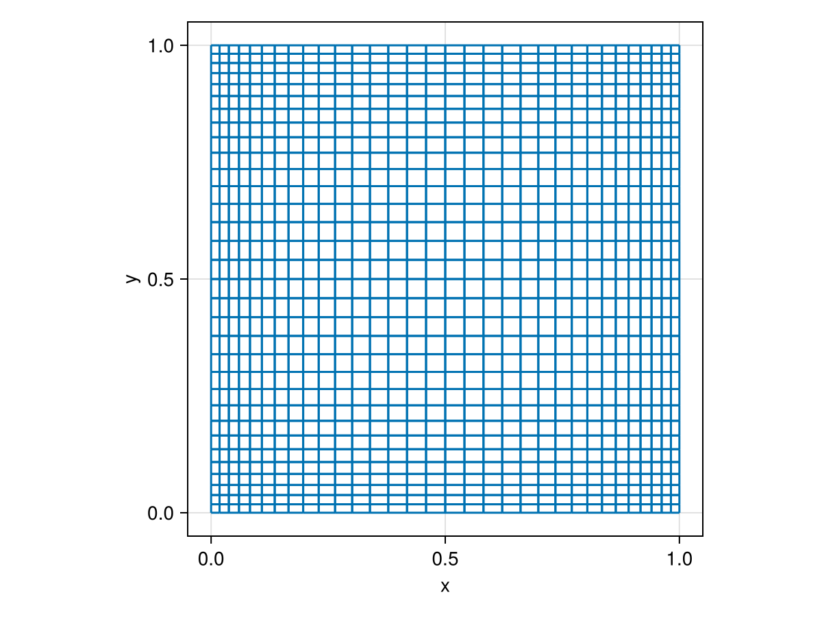

We can now build the setup and assemble operators. A 3D setup is built if we also provide a vector of z-coordinates.

setup = Setup(; x = (ax, ax), boundary_conditions);

Initial conditions

u = velocityfield(setup, (dim, x, y) -> zero(x));

Iteration processors are called after every nupdate time steps. This can be useful for logging, plotting, or saving results. Their respective outputs are later returned by solve_unsteady.

processors = (
    # rtp = realtimeplotter(; setup, plot = fieldplot, nupdate = 50),
    # ehist = realtimeplotter(; setup, plot = energy_history_plot, nupdate = 10),
    # espec = realtimeplotter(; setup, plot = energy_spectrum_plot, nupdate = 10),
    # anim = animator(; setup, path = "$outdir/solution.mkv", nupdate = 20),
    # vtk = vtk_writer(; setup, nupdate = 100, dir = outdir, filename = "solution"),
    # field = fieldsaver(; setup, nupdate = 10),
    log = timelogger(; nupdate = 1000),
);

state, outputs = solve_unsteady(;
    setup,
    start = (; u),
    tlims = (0.0, 10.0),
    params = (; viscosity = 1e-3),
    processors,
);

[ Info: Finished after 350 time steps and 0.9 seconds

Post-process

We may visualize or export the computed fields

Export fields to VTK. The file outdir/solution.vti may be opened for visualization in ParaView. This is particularly useful for inspecting results from 3D simulations.

filename = joinpath(@__DIR__, "output", "solution")
# save_vtk(state; setup, filename)

"/home/runner/work/IncompressibleNavierStokes.jl/IncompressibleNavierStokes.jl/docs/build/examples/generated/output/solution"

Plot velocity

fieldplot(state; setup, fieldname = :velocitynorm)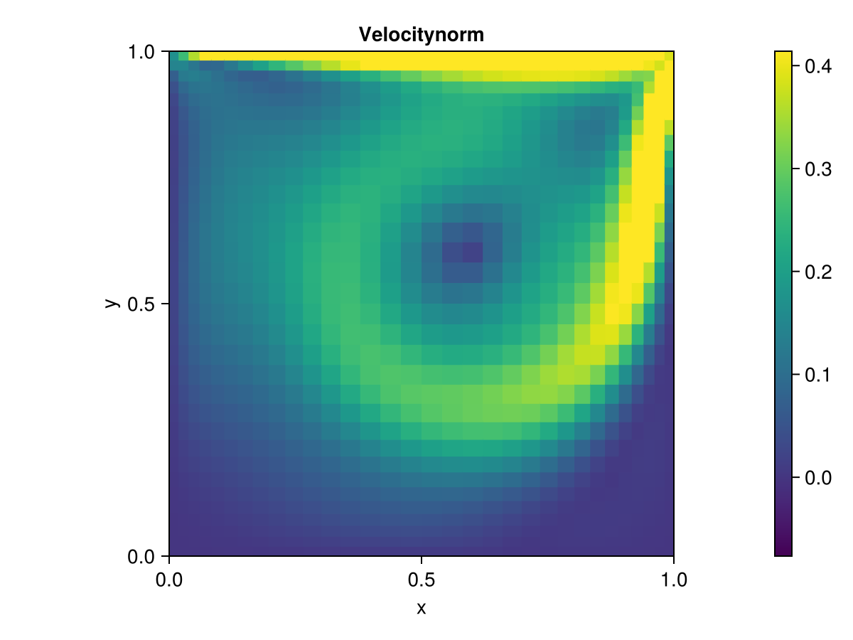

Plot vorticity

fieldplot(state; setup, fieldname = :vorticity)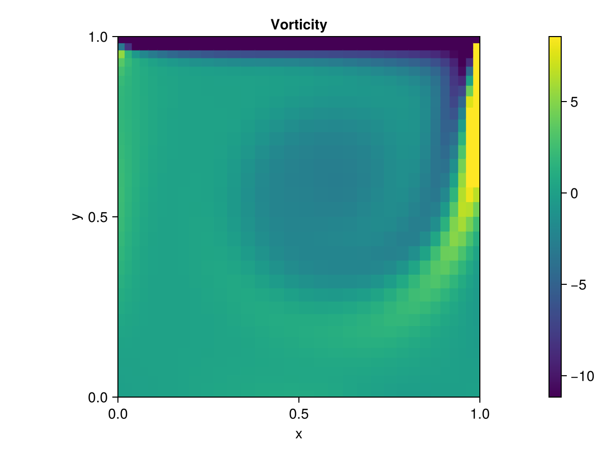

In addition, the named tuple outputs contains quantities from our processors. The logger returns nothing.

# outputs.rtp
# outputs.ehist
# outputs.espec
# outputs.anim
# outputs.vtk
# outputs.field
outputs.log

Copy-pasteable code

Below is the full code for this example stripped of comments and output.

using GLMakie
using IncompressibleNavierStokes

boundary_conditions = (; u = (
    # x left, x right
    (DirichletBC(), DirichletBC()),

    # y bottom, y top
    (DirichletBC(), DirichletBC((1.0, 0.0))),
))

n = 32
ax = tanh_grid(0.0, 1.0, n)
plotgrid(ax, ax)

setup = Setup(; x = (ax, ax), boundary_conditions);

u = velocityfield(setup, (dim, x, y) -> zero(x));

processors = (
    # rtp = realtimeplotter(; setup, plot = fieldplot, nupdate = 50),
    # ehist = realtimeplotter(; setup, plot = energy_history_plot, nupdate = 10),
    # espec = realtimeplotter(; setup, plot = energy_spectrum_plot, nupdate = 10),
    # anim = animator(; setup, path = "$outdir/solution.mkv", nupdate = 20),
    # vtk = vtk_writer(; setup, nupdate = 100, dir = outdir, filename = "solution"),
    # field = fieldsaver(; setup, nupdate = 10),
    log = timelogger(; nupdate = 1000),
);

state, outputs = solve_unsteady(;
    setup,
    start = (; u),
    tlims = (0.0, 10.0),
    params = (; viscosity = 1e-3),
    processors,
);

filename = joinpath(@__DIR__, "output", "solution")
# save_vtk(state; setup, filename)

fieldplot(state; setup, fieldname = :velocitynorm)

fieldplot(state; setup, fieldname = :vorticity)

# outputs.rtp
# outputs.ehist
# outputs.espec
# outputs.anim
# outputs.vtk
# outputs.field
outputs.log

---

This page was generated using Literate.jl.