Rayleigh-Bénard convection (2D)

A hot and a cold plate generate a convection cell in a box.

julia

using CairoMakie
using IncompressibleNavierStokes
# using CUDA, CUDSS

Define observer function to track Nusselt numbers on top and bottom plates.

julia

function nusseltplot(state; setup)
    state isa Observable || (state = Observable(state))
    (; Δ, Δu) = setup
    Δy1 = Δu[2][1:1] |> sum
    Δy2 = Δu[2][(end-1):(end-1)] |> sum

    # Observe Nusselt numbers
    Nu1 = Observable(Point2f[])
    Nu2 = Observable(Point2f[])
    on(state) do (; temp, t)
        dTdy = @. (temp[:, 2] - temp[:, 1]) / Δy1
        Nu = sum((.-dTdy .* Δ[1])[2:(end-1)])
        push!(Nu1[], Point2f(t, Nu))
        dTdy = @. (temp[:, end-1] - temp[:, end-2]) / Δy2
        Nu = sum((.-dTdy .* Δ[1])[2:(end-1)])
        push!(Nu2[], Point2f(t, Nu))
        (Nu1, Nu2) .|> notify ## Update plot
    end

    # Plot Nu history
    fig = Figure()
    ax = Axis(fig[1, 1]; title = "Nusselt number", xlabel = "t", ylabel = "Nu")
    lines!(ax, Nu1; label = "Lower plate")
    lines!(ax, Nu2; label = "Upper plate")
    axislegend(ax)
    on(_ -> autolimits!(ax), Nu2)
    fig
end

nusseltplot (generic function with 1 method)

Define observer function to track average temperature.

julia

function averagetemp(state; setup)
    state isa Observable || (state = Observable(state))
    (; xp, Δ, Ip) = setup
    ix = Ip.indices[1]
    Ty = lift(state) do (; temp)
        Ty = sum(temp[ix, :] .* Δ[1][ix]; dims = 1) ./ sum(Δ[1][ix])
        Array(Ty)[:]
    end
    Ty0 = copy(Ty[])
    yy = Array(xp[2])
    fig = Figure()
    ax = Axis(fig[1, 1]; title = "Average temperature", xlabel = "T", ylabel = "y")
    lines!(ax, Ty0, yy; label = "t = 0")
    lines!(ax, Ty, yy; label = "t = t")
    axislegend(ax)
    on(_ -> autolimits!(ax), Ty)
    fig
end

averagetemp (generic function with 1 method)

Setup

julia

n = 128
setup = Setup(;
    # x = (tanh_grid(0.0, 2.0, 2n, 1.2), tanh_grid(0.0, 1.0, n, 1.2)),
    x = (range(0.0, 2.0, 2n + 1), range(0.0, 1.0, n + 1)),
    boundary_conditions = (;
        u = ((DirichletBC(), DirichletBC()), (DirichletBC(), DirichletBC())),
        temp = ((SymmetricBC(), SymmetricBC()), (DirichletBC(1.0), DirichletBC(0.0))),
    ),
    # backend = CUDABackend()
);

Since the grid is uniform, we can use an FFT/DCT type of solver.

julia

psolver = psolver_transform(setup)

(::IncompressibleNavierStokes.var"#psolve!#121"{Matrix{ComplexF64}, @NamedTuple{uhat::Matrix{ComplexF64}, w::Tuple{Vector{ComplexF64}, Vector{ComplexF64}}, winv::Tuple{Vector{ComplexF64}, Vector{ComplexF64}}, perm::Tuple{Vector{Int64}, Vector{Int64}}, perminv::Tuple{Vector{Int64}, Vector{Int64}}}, Matrix{Float64}, Tuple{Vector{Float64}, Vector{Float64}}, Tuple{Bool, Bool}, Int64, CartesianIndices{2, Tuple{UnitRange{Int64}, UnitRange{Int64}}}}) (generic function with 1 method)

Initial conditions

julia

start = (;
    u = velocityfield(setup, (dim, x, y) -> zero(x); psolver),
    temp = temperaturefield(setup, (x, y) -> one(y) / 2 + max(sinpi(20 * x) / 100, 0)),
);

Solve equation

julia

state, outputs = solve_unsteady(;
    force! = boussinesq!, # Solve the Boussinesq equations
    setup,
    start,
    tlims = (0.0, 20.0),
    psolver,
    params = (;
        viscosity = 2.5e-4,
        gravity = 1.0,
        gdir = 2,
        conductivity = 2.5e-4,
        dodissipation = true,
    ),
    processors = (;
        rtp = realtimeplotter(;
            setup,
            fieldname = :temperature,
            colorrange = (0.0, 1.0),
            size = (600, 350),
            colormap = :seaborn_icefire_gradient,
            nupdate = 20,
        ),
        nusselt = realtimeplotter(;
            setup,
            plot = nusseltplot,
            displayfig = false,
            nupdate = 20,
        ),
        avg = realtimeplotter(;
            setup,
            plot = averagetemp,
            displayfig = false,
            nupdate = 50,
        ),
        log = timelogger(; nupdate = 1000),
    ),
);

[ Info: Finished after 564 time steps and 8.7 seconds

Nusselt numbers

julia

outputs.nusselt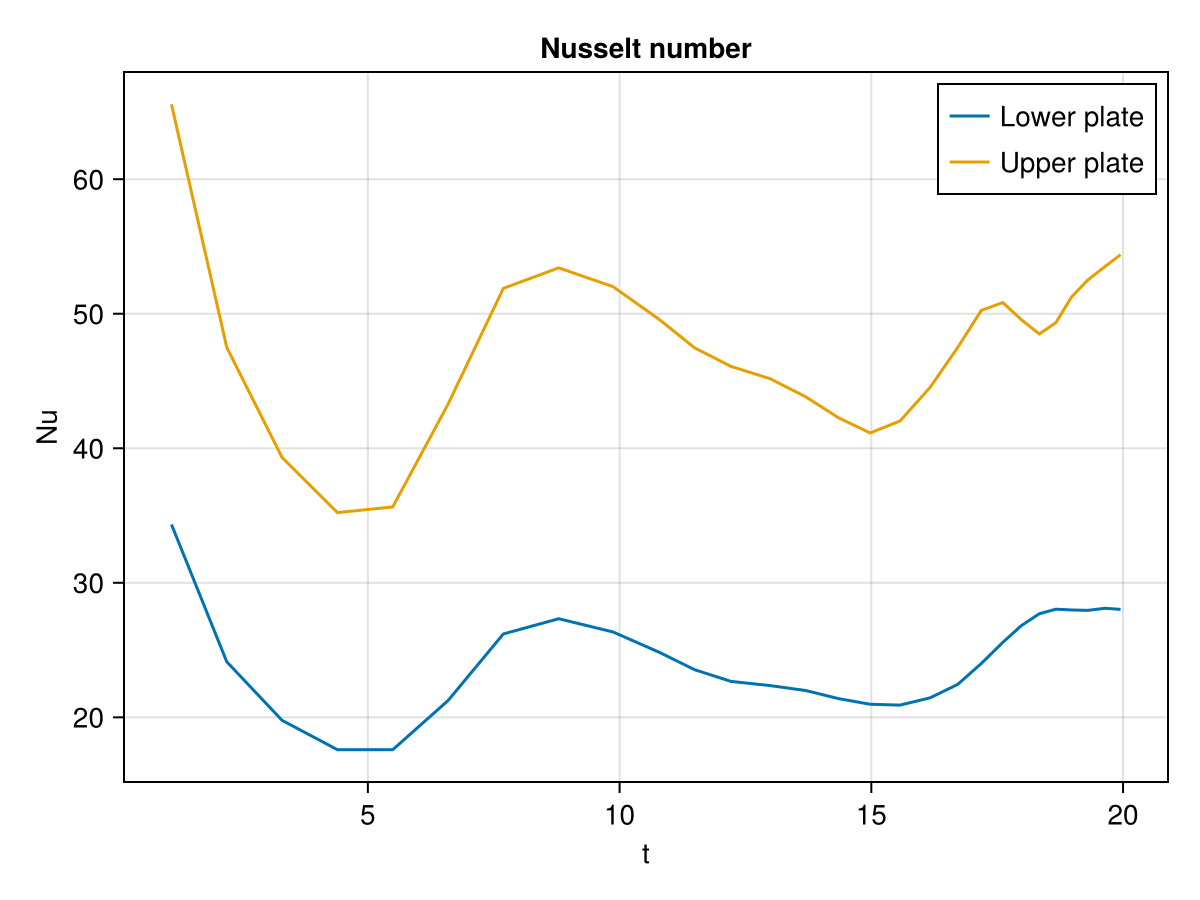

Average temperature

julia

outputs.avg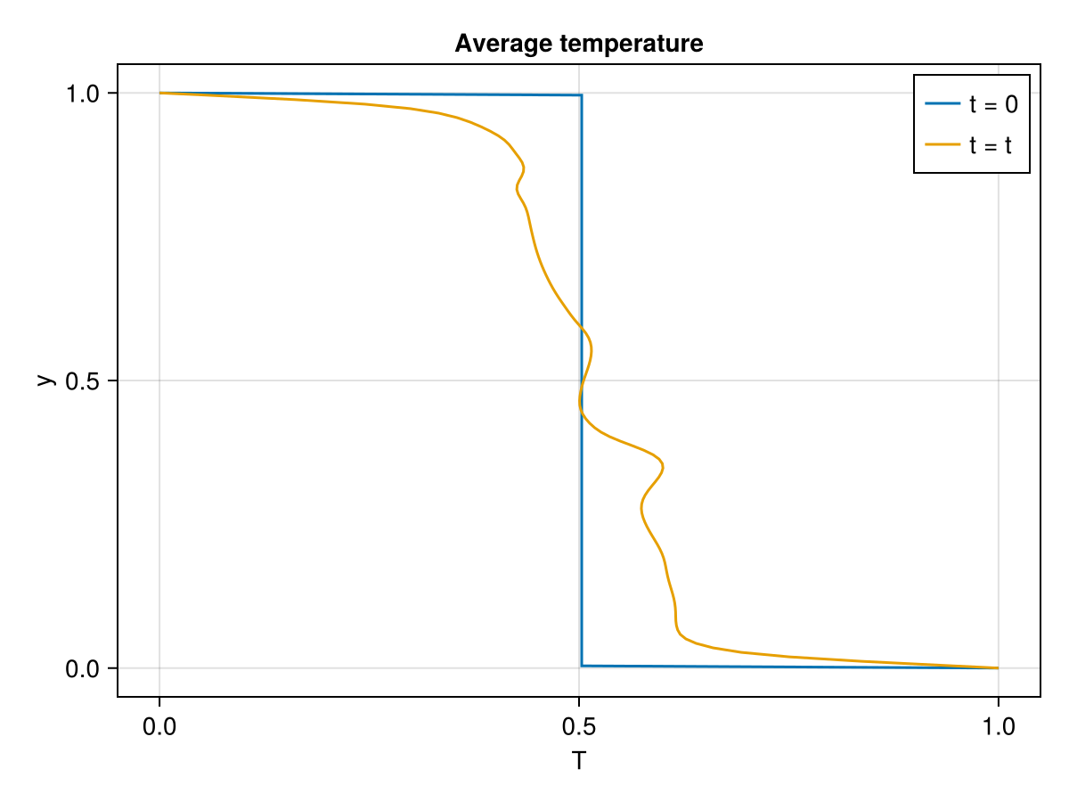

Copy-pasteable code

Below is the full code for this example stripped of comments and output.

julia

using WGLMakie
using IncompressibleNavierStokes
# using CUDA, CUDSS

function nusseltplot(state; setup)
    state isa Observable || (state = Observable(state))
    (; Δ, Δu) = setup
    Δy1 = Δu[2][1:1] |> sum
    Δy2 = Δu[2][(end-1):(end-1)] |> sum

    # Observe Nusselt numbers
    Nu1 = Observable(Point2f[])
    Nu2 = Observable(Point2f[])
    on(state) do (; temp, t)
        dTdy = @. (temp[:, 2] - temp[:, 1]) / Δy1
        Nu = sum((.-dTdy .* Δ[1])[2:(end-1)])
        push!(Nu1[], Point2f(t, Nu))
        dTdy = @. (temp[:, end-1] - temp[:, end-2]) / Δy2
        Nu = sum((.-dTdy .* Δ[1])[2:(end-1)])
        push!(Nu2[], Point2f(t, Nu))
        (Nu1, Nu2) .|> notify ## Update plot
    end

    # Plot Nu history
    fig = Figure()
    ax = Axis(fig[1, 1]; title = "Nusselt number", xlabel = "t", ylabel = "Nu")
    lines!(ax, Nu1; label = "Lower plate")
    lines!(ax, Nu2; label = "Upper plate")
    axislegend(ax)
    on(_ -> autolimits!(ax), Nu2)
    fig
end

function averagetemp(state; setup)
    state isa Observable || (state = Observable(state))
    (; xp, Δ, Ip) = setup
    ix = Ip.indices[1]
    Ty = lift(state) do (; temp)
        Ty = sum(temp[ix, :] .* Δ[1][ix]; dims = 1) ./ sum(Δ[1][ix])
        Array(Ty)[:]
    end
    Ty0 = copy(Ty[])
    yy = Array(xp[2])
    fig = Figure()
    ax = Axis(fig[1, 1]; title = "Average temperature", xlabel = "T", ylabel = "y")
    lines!(ax, Ty0, yy; label = "t = 0")
    lines!(ax, Ty, yy; label = "t = t")
    axislegend(ax)
    on(_ -> autolimits!(ax), Ty)
    fig
end

n = 128
setup = Setup(;
    # x = (tanh_grid(0.0, 2.0, 2n, 1.2), tanh_grid(0.0, 1.0, n, 1.2)),
    x = (range(0.0, 2.0, 2n + 1), range(0.0, 1.0, n + 1)),
    boundary_conditions = (;
        u = ((DirichletBC(), DirichletBC()), (DirichletBC(), DirichletBC())),
        temp = ((SymmetricBC(), SymmetricBC()), (DirichletBC(1.0), DirichletBC(0.0))),
    ),
    # backend = CUDABackend()
);

psolver = psolver_transform(setup)

start = (;
    u = velocityfield(setup, (dim, x, y) -> zero(x); psolver),
    temp = temperaturefield(setup, (x, y) -> one(y) / 2 + max(sinpi(20 * x) / 100, 0)),
);

state, outputs = solve_unsteady(;
    force! = boussinesq!, # Solve the Boussinesq equations
    setup,
    start,
    tlims = (0.0, 20.0),
    psolver,
    params = (;
        viscosity = 2.5e-4,
        gravity = 1.0,
        gdir = 2,
        conductivity = 2.5e-4,
        dodissipation = true,
    ),
    processors = (;
        rtp = realtimeplotter(;
            setup,
            fieldname = :temperature,
            colorrange = (0.0, 1.0),
            size = (600, 350),
            colormap = :seaborn_icefire_gradient,
            nupdate = 20,
        ),
        nusselt = realtimeplotter(;
            setup,
            plot = nusseltplot,
            displayfig = false,
            nupdate = 20,
        ),
        avg = realtimeplotter(;
            setup,
            plot = averagetemp,
            displayfig = false,
            nupdate = 50,
        ),
        log = timelogger(; nupdate = 1000),
    ),
);

outputs.nusselt

outputs.avg

This page was generated using Literate.jl.

Rayleigh-Bénard convection (2D) ​

Copy-pasteable code ​

Rayleigh-Bénard convection (2D)

Copy-pasteable code