Spatial discretization

the $d$ spatial dimensions are indexed by $\alpha \in \{1,\dots ,d\}$. The $\alpha$-th unit vector is denoted $e_{\alpha }=(e_{\alpha \beta }{)}_{\beta =1}^d$, where the Kronecker symbol $e_{\alpha \beta }$ is $1$ if $\alpha =\beta$ and $0$ otherwise. We note $h_{\alpha }=e_{\alpha }/2$. The Cartesian index $I=(I_1,\dots ,I_d)$ is used to avoid repeating terms and equations $d$ times, where $I_{\alpha }$ is a scalar index (typically one of $i$, $j$, and $k$ in common notation). This notation is dimension-agnostic, since we can write $u_I$ instead of $u_{ij}$ in 2D or $u_{ijk}$ in 3D. In our Julia implementation of the solver we use the same Cartesian notation (u[I] instead of u[i, j] or u[i, j, k]).

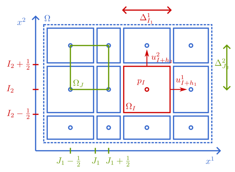
For the discretization scheme, we use a staggered Cartesian grid as proposed by Harlow and Welch [12]. Consider a rectangular domain $\mathrm{\Omega }=\prod _{\alpha =1}^d[a_{\alpha },b_{\alpha }]$, where $a_{\alpha }<b_{\alpha }$ are the domain boundaries and $\prod$ is a Cartesian product. Let $\mathrm{\Omega }=\bigcup _{I\in \mathcal{I}}{\mathrm{\Omega }}_I$ be a partitioning of $\mathrm{\Omega }$, where $\mathcal{I}=\prod _{\alpha =1}^d\{\frac{1}{2},2-\frac{1}{2},\dots ,N_{\alpha }-\frac{1}{2}\}$ are volume center indices, $N=(N_1,\dots ,N_d)\in {\mathbb{N}}^d$ are the number of volumes in each dimension, ${\mathrm{\Omega }}_I=\prod _{\alpha =1}^d{\mathrm{\Delta }}_{I_{\alpha }}^{\alpha }$ is a finite volume, ${\mathrm{\Gamma }}_I^{\alpha }={\mathrm{\Omega }}_{I-h_{\alpha }}\cap {\mathrm{\Omega }}_{I+h_{\alpha }}=\prod _{\beta \ne \alpha }{\mathrm{\Delta }}_{I_{\beta }}^{\beta }$ is a volume face, ${\mathrm{\Delta }}_i^{\alpha }=[x_{i-\frac{1}{2}}^{\alpha },x_{i+\frac{1}{2}}^{\alpha }]$ is a volume edge, $x_0^{\alpha },\dots ,x_{N_{\alpha }}^{\alpha }$ are volume boundary coordinates, and $x_i^{\alpha }=\frac{1}{2}(x_{i-\frac{1}{2}}^{\alpha }+x_{i+\frac{1}{2}}^{\alpha })$ for $i\in \{1/2,\dots ,N_{\alpha }-1/2\}$ are volume center coordinates. We also define the operator ${\delta }_{\alpha }$ which maps a discrete scalar field $\phi =({\phi }_I{)}_I$ to

$$({\delta }_{\alpha }\phi {)}_I=\frac{{\phi }_{I+h_{\alpha }}-{\phi }_{I-h_{\alpha }}}{|{\mathrm{\Delta }}_{I_{\alpha }}^{\alpha }|}.$$

It can be interpreted as a discrete equivalent of the continuous operator $\frac{\partial }{\partial x^{\alpha }}$. All the above definitions are extended to be valid in volume centers $I\in \mathcal{I}$, volume faces $I\in \mathcal{I}+h_{\alpha }$, or volume corners $I\in \mathcal{I}+\sum _{\alpha =1}^d{h}_{\alpha }$. The discretization is illustrated below:

Finite volume discretization of the Navier-Stokes equations

We now define the unknown degrees of freedom. The average pressure in ${\mathrm{\Omega }}_I$, $I\in \mathcal{I}$ is approximated by the quantity $p_I(t)$. The average $\alpha$-velocity on the face ${\mathrm{\Gamma }}_I^{\alpha }$, $I\in \mathcal{I}+h_{\alpha }$ is approximated by the quantity $u_I^{\alpha }(t)$. Note how the pressure $p$ and the $d$ velocity fields $u^{\alpha }$ are each defined in their own canonical positions $x_I$ and $x_{I+h_{\alpha }}$ for $I\in \mathcal{I}$. In the following, we derive equations for these unknowns.

Using the pressure control volume $\mathcal{O}={\mathrm{\Omega }}_I$ with $I\in \mathcal{I}$ in the mass integral constraint and approximating the face integrals with the mid-point quadrature rule ${\int }_{{\mathrm{\Gamma }}_I}u\mathrm{d}\mathrm{\Gamma }\approx |{\mathrm{\Gamma }}_I|u_I$ results in the discrete divergence-free constraint

$$\sum _{\alpha =1}^d({\delta }_{\alpha }{u}^{\alpha }{)}_I=0.$$

Note how dividing by the volume size results in a discrete equation resembling the continuous one (since $|{\mathrm{\Omega }}_I|=|{\mathrm{\Gamma }}_I^{\alpha }||{\mathrm{\Delta }}_{I_{\alpha }}^{\alpha }|$).

Similarly, choosing an $\alpha$-velocity control volume $\mathcal{O}={\mathrm{\Omega }}_I$ with $I\in \mathcal{I}+h_{\alpha }$ in the integral momentum equation, approximating the volume- and face integrals using the mid-point quadrature rule, and replacing remaining spatial derivatives in the diffusive term with a finite difference approximation gives the discrete momentum equations

$$\frac{\mathrm{d}}{\mathrm{d}t}{u}_I^{\alpha }=-\sum _{\beta =1}^d({\delta }_{\beta }(u^{\alpha }{u}^{\beta }){)}_I+\nu \sum _{\beta =1}^d({\delta }_{\beta }{\delta }_{\beta }{u}^{\alpha }{)}_I+f^{\alpha }(x_I)-({\delta }_{\alpha }p{)}_I.$$

where we made the assumption that $f$ is constant in time for simplicity. The outer discrete derivative in $({\delta }_{\beta }{\delta }_{\beta }{u}^{\alpha }{)}_I$ is required at the position $I$, which means that the inner derivative is evaluated as $({\delta }_{\beta }{u}^{\alpha }{)}_{I+h_{\beta }}$ and $({\delta }_{\beta }{u}^{\alpha }{)}_{I-h_{\beta }}$, thus requiring $u_{I-2h_{\beta }}^{\alpha }$, $u_I^{\alpha }$, and $u_{I+2h_{\beta }}^{\alpha }$, which are all in their canonical positions. The two velocity components in the convective term $u^{\alpha }{u}^{\beta }$ are required at the positions $I-h_{\beta }$ and $I+h_{\beta }$, which are outside the canonical positions. Their value at the required position is obtained using averaging with weights $1/2$ for the $\alpha$-component and with linear interpolation for the $\beta$-component. This preserves the skew-symmetry of the convection operator, such that energy is conserved (in the convective term) [13].

Boundary conditions

Storage convention

We use the column-major convention (Julia, MATLAB, Fortran), and not the row-major convention (Python, C). Thus the $x^1$-index $i$ will vary for one whole cycle in the vectors before the $x^2$-index $j$, $x^3$ index $k$, and component-index $\alpha$ are incremented, e.g. $u_h=(u_{(1,1,1)}^1,u_{(2,1,1)}^1,\dots u_{(N_{u^3}(1),N_{u^3}(2),N_{u^3}(3))}^3)$ in 3D.

Fourth order accurate discretization

The above discretization is second order accurate. A fourth order accurate discretization can be obtained by judiciously combining the second order discretization with itself on a grid with three times larger cells in each dimension [13] [14]. The coarse discretization is identical, but the mass equation is derived for the three times coarser control volume

$${\mathrm{\Omega }}_I^3=\bigcup _{\alpha =1}^d{\mathrm{\Omega }}_{I-e_{\alpha }}\cup {\mathrm{\Omega }}_I\cup {\mathrm{\Omega }}_{I+e_{\alpha }},$$

while the momentum equation is derived for its shifted variant ${\mathrm{\Omega }}_{I+h_{\alpha }}^3$. The resulting fourth order accurate equations are given by

$$\sum _{\alpha =1}^d({\delta }_{\alpha }{u}^{\alpha }{)}_I-\frac{|{\mathrm{\Omega }}_I^3|}{3^{2+d}|{\mathrm{\Omega }}_I|}\sum _{\alpha =1}^d({\delta }_{\alpha }^3{u}^{\alpha }{)}_I=0$$

and

$$\frac{\mathrm{d}}{\mathrm{d}t}{u}_I^{\alpha }=-\sum _{\beta =1}^d({\delta }_{\beta }(u^{\alpha }{u}^{\beta }){)}_I+\nu \sum _{\beta =1}^d({\delta }_{\beta }{\delta }_{\beta }{u}^{\alpha }{)}_I+f^{\alpha }(x_I)-({\delta }_{\alpha }p{)}_I+\text{fourth order},$$

where

$$({\delta }_{\alpha }^3\phi {)}_I=\frac{{\phi }_{I+3h_{\alpha }}-{\phi }_{I-3h_{\alpha }}}{{\mathrm{\Delta }}_{I_{\alpha }-1}^{\alpha }+{\mathrm{\Delta }}_{I_{\alpha }}^{\alpha }+{\mathrm{\Delta }}_{I_{\alpha }+1}^{\alpha }}.$$

Matrix representation

We can write the mass and momentum equations in matrix form. We will use the same matrix notation for the second- and fourth order accurate discretizations. The discrete mass equation becomes

$$M{u}_h+y_M=0,$$

where $M$ is the discrete divergence operator and $y_M$ contains the boundary value contributions of the velocity to the divergence field.

The discrete momentum equations become

$$\begin{array}{rl}\frac{\mathrm{d}{u}_h}{\mathrm{d}t}& =-C(u_h)+\nu (D{u}_h+y_D)+f_h-(G{p}_h+y_G)\\ & =F(u_h)-(G{p}_h+y_G),\end{array}$$

where $C$ is she convection operator (including boundary contributions), $D$ is the diffusion operator, $y_D$ is boundary contribution to the diffusion term, $G=W_u^{-1}{M}^{\mathsf{T}}W$ is the pressure gradient operator, $y_G$ contains the boundary contribution of the pressure to the pressure gradient (only non-zero for pressure boundary conditions), $W_u$ is a diagonal matrix containing the velocity volume sizes $|{\mathrm{\Omega }}_{I+\delta (\alpha )/2}|$, and $W$ is a diagonal matrix containing the reference volume sizes $|{\mathrm{\Omega }}_I|$. The term $F$ refers to all the forces except for the pressure gradient.

Volume normalization

All the operators have been divided by the velocity volume sizes. As a result, the operators have the same units as their continuous counterparts.

Discrete pressure Poisson equation

Instead of directly discretizing the continuous pressure Poisson equation, we will rededuce it in the discrete setting, thus aiming to preserve the discrete divergence freeness instead of the continuous one. Applying the discrete divergence operator $M$ to the discrete momentum equations yields the discrete pressure Poisson equation

$$L{p}_h=WM(F(u_h)-y_G)+W\frac{\mathrm{d}{y}_M}{\mathrm{d}t},$$

where $L=WMG=WM{W}_u^{-1}{M}^{\mathsf{T}}W$ is a discrete Laplace operator. It is positive symmetric.

Unsteady Dirichlet boundary conditions

If the equations are prescribed with unsteady Dirichlet boundary conditions, for example an inflow that varies with time, the term $\frac{\mathrm{d}{y}_M}{\mathrm{d}t}$ will be non-zero. If this term is not known exactly, for example if the next value of the inflow is unknown at the time of the current value, it must be computed using past values of of the velocity inflow only, for example $\frac{\mathrm{d}{y}_M}{\mathrm{d}t}\approx (y_M(t)-y_M(t-\mathrm{\Delta }t))/\mathrm{\Delta }t$ for some $\mathrm{\Delta }t$.

Uniqueness of pressure field

Unless pressure boundary conditions are present, the pressure is only determined up to a constant, as $L$ will have an eigenvalue of zero. Since only the gradient of the pressure appears in the equations, we can set the unknown constant to zero without affecting the velocity field.

Pressure projection

The pressure field $p_h$ can be seen as a Lagrange multiplier enforcing the constraint of discrete divergence freeness. It is also possible to write the momentum equations without the pressure by explicitly solving the discrete Poisson equation:

$$p_h=L^{-1}WM(F(u_h)-y_G)+L^{-1}W\frac{\mathrm{d}{y}_M}{\mathrm{d}t}.$$

The momentum equations then become

$$\frac{\mathrm{d}{u}_h}{\mathrm{d}t}=(I-G{L}^{-1}WM)(F(u_h)-y_G)-G{L}^{-1}W\frac{\mathrm{d}{y}_M}{\mathrm{d}t}.$$

The matrix $(I-G{L}^{-1}WM)$ is a projector onto the space of discretely divergence free velocities. However, using this formulation would require an efficient way to perform the projection without assembling the operator matrix $L^{-1}$, which would be very costly.

Discrete output quantities

Kinetic energy

The local kinetic energy is defined by $k=\frac{1}{2}\parallel u{\parallel }_2^2=\frac{1}{2}\sum _{\alpha =1}^d{u}^{\alpha }{u}^{\alpha }$. On the staggered grid however, the different velocity components are not located at the same point. We will therefore interpolate the velocity to the pressure point before summing the squares.

Vorticity

In 2D, the vorticity is a scalar. We define it as

$$\omega =-{\delta }^2{u}^1+{\delta }^1{u}^2.$$

The 3D vorticity is a vector field $({\omega }^1,{\omega }^2,{\omega }^3)$. Noting ${\alpha }^{+}={\mathrm{mod}}_3(\alpha +1)$ and ${\alpha }^{-}={\mathrm{mod}}_3(\alpha -1)$, the vorticity is defined as through

$${\omega }^{\alpha }=-{\delta }^{{\alpha }^{-}}{u}^{{\alpha }^{+}}+{\delta }^{{\alpha }^{+}}{u}^{{\alpha }^{-}}.$$

Stream function

In 2D, the stream function is defined at the corners with the vorticity. Integrating the stream function Poisson equation over the vorticity volume yields

$$\begin{array}{rl}-{\int }_{{\mathrm{\Omega }}_{I+h_1+h_2}}\omega \mathrm{d}\mathrm{\Omega }& ={\int }_{{\mathrm{\Omega }}_{I+h_1+h_2}}{\mathrm{\nabla }}^2\psi \mathrm{d}\mathrm{\Omega }\\ & ={\int }_{{\mathrm{\Gamma }}_{I+e_1+h_2}^1}\frac{\partial \psi }{\partial x^1}\mathrm{d}\mathrm{\Gamma }-{\int }_{{\mathrm{\Gamma }}_{I+h_2}^1}\frac{\partial \psi }{\partial x^1}\mathrm{d}\mathrm{\Gamma }\\ & +{\int }_{{\mathrm{\Gamma }}_{I+h_1+e_2}^2}\frac{\partial \psi }{\partial x^2}\mathrm{d}\mathrm{\Gamma }-{\int }_{{\mathrm{\Gamma }}_{I+h_1}^2}\frac{\partial \psi }{\partial x^2}\mathrm{d}\mathrm{\Gamma }.\end{array}$$

Replacing the integrals with the mid-point quadrature rule and the spatial derivatives with central finite differences yields the discrete Poisson equation for the stream function at the vorticity point:

$$\begin{array}{rl}\left|{\mathrm{\Gamma }}_{I+h_1+h_2}^1\right|(\frac{{\psi }_{I+3/h_1+h_2}-{\psi }_{I+h_1+h_2}}{x_{I_1+3/2}^1-x_{I_1+1/2}^1}-\frac{{\psi }_{I+h_1+h_2}-{\psi }_{I-h_1+h_2}}{x_{I_1+1/2}^1-x_{I_1-1/2}^1})& +\\ \left|{\mathrm{\Gamma }}_{I+h_1+h_2}^2\right|(\frac{{\psi }_{I+h_1+3h_2}-{\psi }_{I+h_1+h_2}}{x_{I_1+3/2}^2-x_{I_1+1/2}^2}-\frac{{\psi }_{I+h_1+h_2}-{\psi }_{I+h_1-h_2}}{x_{I_2+1/2}^2-x_{I_2-1/2}^2})& =\\ \left|{\mathrm{\Omega }}_{I+h_1+h_2}\right|{\omega }_{I+h_1+h_2}& \end{array}$$