Convergence study: Taylor-Green vortex (2D)

In this example we consider the Taylor-Green vortex. In 2D, it has an analytical solution, given by

$$\begin{array}{rl}{u}^1(x,y,t)& =-\sin (x)\cos (y){\mathrm{e}}^{-2t\nu }\\ u^2(x,y,t)& =+\cos (x)\sin (y){\mathrm{e}}^{-2t\nu }\end{array}$$

This allows us to test the convergence of our solver.

using CairoMakie
using IncompressibleNavierStokes
using LinearAlgebra

Output directory

outdir = joinpath(@__DIR__, "output", "TaylorGreenVortex2D")
ispath(outdir) || mkpath(outdir)

"/home/runner/work/IncompressibleNavierStokes.jl/IncompressibleNavierStokes.jl/docs/build/examples/generated/output/TaylorGreenVortex2D"

Convergence

"""
Compare numerical solution with analytical solution at final time.
"""
function compute_convergence(; D, nlist, lims, viscosity, tlims, uref)
    T = typeof(lims[1])
    e = zeros(T, length(nlist))
    for (i, n) in enumerate(nlist)
        @info "Computing error for n = $n"
        x = ntuple(α -> LinRange(lims..., n + 1), D)
        setup = Setup(;
            x,
            boundary_conditions = (;
                u = ((PeriodicBC(), PeriodicBC()), (PeriodicBC(), PeriodicBC())),
            ),
        )
        ustart = velocityfield(setup, (dim, x...) -> uref(dim, x..., tlims[1]), tlims[1];)
        ut = velocityfield(
            setup,
            (dim, x...) -> uref(dim, x..., tlims[2]),
            tlims[2];
            doproject = false,
        )
        (; u, t), outputs =
            solve_unsteady(; setup, start = (; u = ustart), tlims, params = (; viscosity))
        (; Ip) = setup
        a = sum(abs2, u[Ip, :] - ut[Ip, :])
        b = sum(abs2, ut[Ip, :])
        e[i] = sqrt(a) / sqrt(b)
    end
    e
end

Main.compute_convergence

Analytical solution for 2D Taylor-Green vortex

solution(viscosity) =
    (dim, x, y, t) -> (dim == 1 ? -sin(x) * cos(y) : cos(x) * sin(y)) * exp(-2t * viscosity)

solution (generic function with 1 method)

Compute error for different resolutions

viscosity = 5e-4
nlist = [2, 4, 8, 16, 32, 64, 128, 256]
e = compute_convergence(;
    D = 2,
    nlist,
    lims = (0.0, 2π),
    viscosity,
    tlims = (0.0, 2.0),
    uref = solution(viscosity),
)

8-element Vector{Float64}:
 0.42426560520867174
 0.0003789328383510445
 0.00010072266505864668
 2.5570665387178272e-5
 6.417292500357841e-6
 1.60586621087271e-6
 4.0156305742092024e-7
 1.0039679684863276e-7

Plot convergence

let
    fig = Figure()
    ax = Axis(
        fig[1, 1];
        xscale = log10,
        yscale = log10,
        xticks = nlist,
        xlabel = "n",
        title = "Relative error",
    )
    scatterlines!(ax, nlist, e; label = "Data")
    lines!(ax, collect(extrema(nlist)), n -> n^-2.0; linestyle = :dash, label = "n^-2")
    axislegend(ax)
    save(joinpath(outdir, "convergence.png"), fig)
    fig
end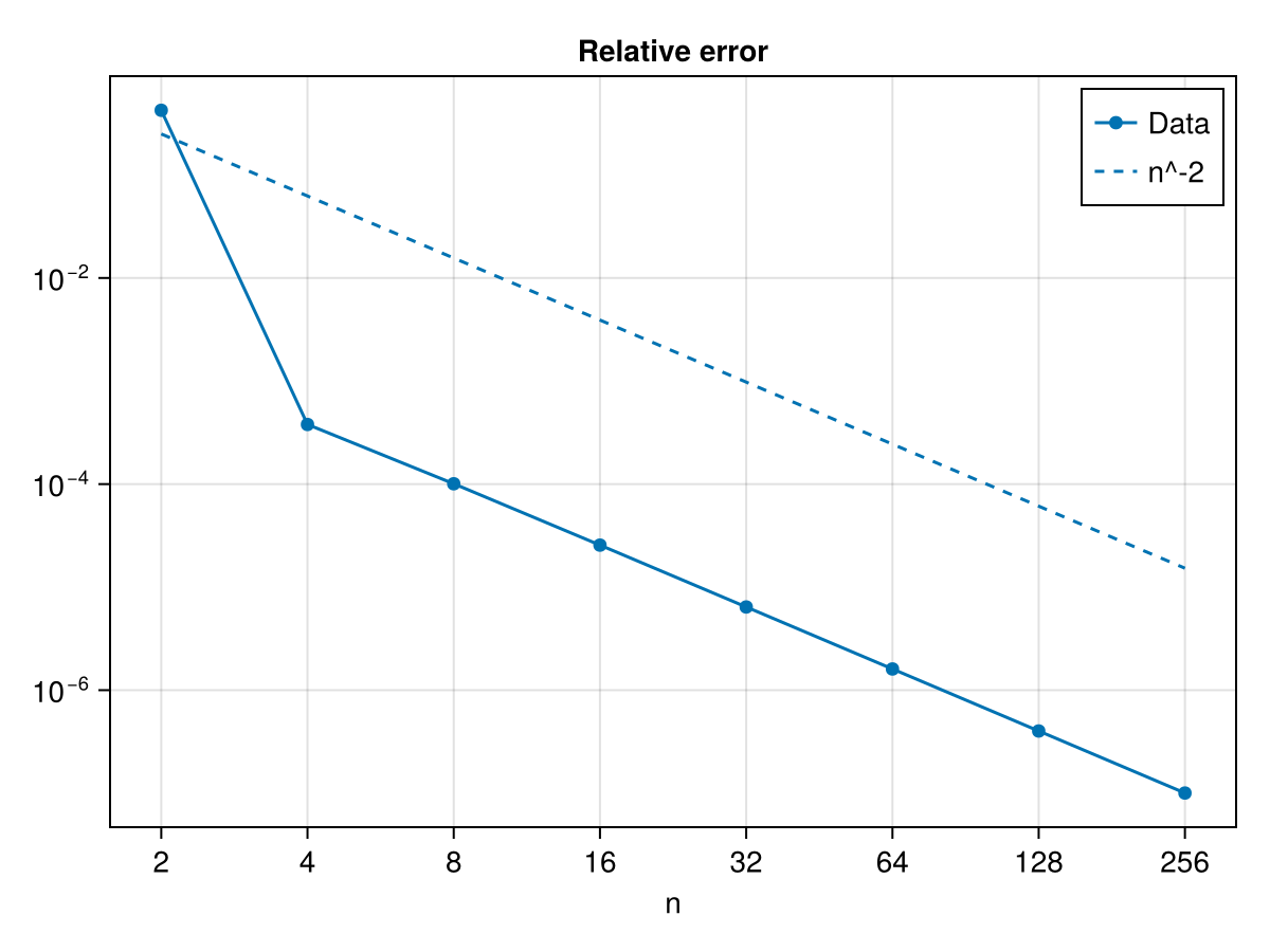

Copy-pasteable code

Below is the full code for this example stripped of comments and output.

using WGLMakie
using IncompressibleNavierStokes
using LinearAlgebra

outdir = joinpath(@__DIR__, "output", "TaylorGreenVortex2D")
ispath(outdir) || mkpath(outdir)

"""
Compare numerical solution with analytical solution at final time.
"""
function compute_convergence(; D, nlist, lims, viscosity, tlims, uref)
    T = typeof(lims[1])
    e = zeros(T, length(nlist))
    for (i, n) in enumerate(nlist)
        @info "Computing error for n = $n"
        x = ntuple(α -> LinRange(lims..., n + 1), D)
        setup = Setup(;
            x,
            boundary_conditions = (;
                u = ((PeriodicBC(), PeriodicBC()), (PeriodicBC(), PeriodicBC())),
            ),
        )
        ustart = velocityfield(setup, (dim, x...) -> uref(dim, x..., tlims[1]), tlims[1];)
        ut = velocityfield(
            setup,
            (dim, x...) -> uref(dim, x..., tlims[2]),
            tlims[2];
            doproject = false,
        )
        (; u, t), outputs =
            solve_unsteady(; setup, start = (; u = ustart), tlims, params = (; viscosity))
        (; Ip) = setup
        a = sum(abs2, u[Ip, :] - ut[Ip, :])
        b = sum(abs2, ut[Ip, :])
        e[i] = sqrt(a) / sqrt(b)
    end
    e
end

solution(viscosity) =
    (dim, x, y, t) -> (dim == 1 ? -sin(x) * cos(y) : cos(x) * sin(y)) * exp(-2t * viscosity)

viscosity = 5e-4
nlist = [2, 4, 8, 16, 32, 64, 128, 256]
e = compute_convergence(;
    D = 2,
    nlist,
    lims = (0.0, 2π),
    viscosity,
    tlims = (0.0, 2.0),
    uref = solution(viscosity),
)

let
    fig = Figure()
    ax = Axis(
        fig[1, 1];
        xscale = log10,
        yscale = log10,
        xticks = nlist,
        xlabel = "n",
        title = "Relative error",
    )
    scatterlines!(ax, nlist, e; label = "Data")
    lines!(ax, collect(extrema(nlist)), n -> n^-2.0; linestyle = :dash, label = "n^-2")
    axislegend(ax)
    save(joinpath(outdir, "convergence.png"), fig)
    fig
end

---

This page was generated using Literate.jl.