Unsteady actuator case - 2D

In this example, an unsteady inlet velocity profile at encounters a wind turbine blade in a wall-less domain. The blade is modeled as a uniform body force on a thin rectangle.

Packages

A Makie plotting backend is needed for plotting. GLMakie creates an interactive window (useful for real-time plotting), but does not work when building this example on GitHub. CairoMakie makes high-quality static vector-graphics plots.

using CairoMakie
using IncompressibleNavierStokes

Setup

A 2D grid is a Cartesian product of two vectors

n = 40
x = LinRange(0.0, 10.0, 5n + 1), LinRange(-2.0, 2.0, 2n + 1)
plotgrid(x...; figure = (; size = (600, 300)))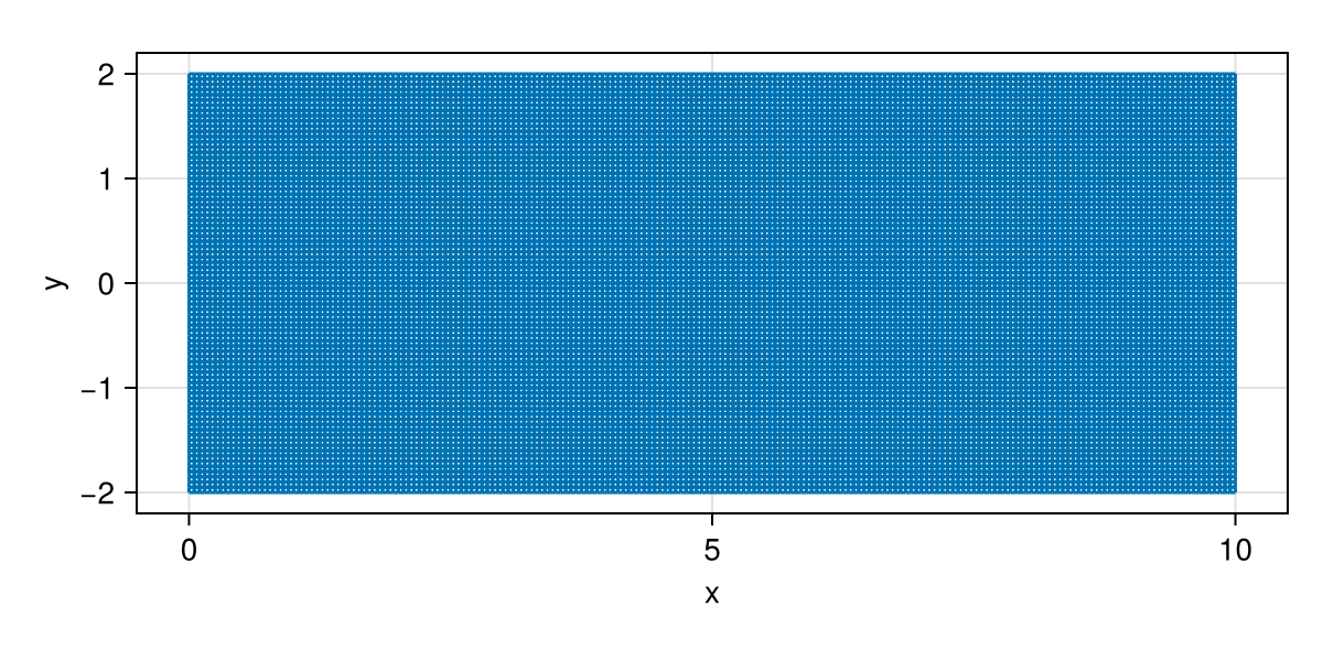

Boundary conditions

inflow(dim, x, y, t) = sinpi(sinpi(t / 6) / 6 + (dim == 1) / 2)
boundary_conditions =
    (; u = ((DirichletBC(inflow), PressureBC()), (PressureBC(), PressureBC())))

(u = ((DirichletBC{typeof(Main.inflow)}(Main.inflow), PressureBC()), (PressureBC(), PressureBC())),)

Build setup

setup = Setup(; x, boundary_conditions);

Actuator body force: A thrust coefficient Cₜ distributed over a thin rectangle

xc, yc = 2.0, 0.0 # Disk center
D = 1.0           # Disk diameter
δ = 0.11          # Disk thickness
C = 0.2           # Thrust coefficient
c = C / (D * δ)   # Normalize
inside(x, y) = abs(x - xc) ≤ δ / 2 && abs(y - yc) ≤ D / 2
f(dim, x, y) = -c * (dim == 1) * inside(x, y)

f (generic function with 1 method)

This is the right-hand side force in the momentum equation By default, it is just navierstokes!. Here we add a pre-computed body force.

function force!(f, state, t; setup, cache, viscosity)
    navierstokes!(f, state, t; setup, cache, viscosity)
    f.u .+= cache.bodyforce
end

force! (generic function with 1 method)

Tell IncompressibleNavierStokes how to prepare the cache for force!. The cache is created before time stepping begins.

IncompressibleNavierStokes.get_cache(::typeof(force!), setup) =
    (; bodyforce = velocityfield(setup, f; doproject = false))

Initial conditions (extend inflow)

u = velocityfield(setup, (dim, x, y) -> inflow(dim, x, y, 0.0));

Solve unsteady problem

@profview

state, outputs = solve_unsteady(;
    setup,
    force!,
    params = (; viscosity = 0.01),
    start = (; u),
    tlims = (0.0, 12e0),
    processors = (
        rtp = realtimeplotter(; setup, size = (600, 300), nupdate = 5),
        log = timelogger(; nupdate = 100),
    ),
);

[ Info: t = 1.40625	Δt = 0.014	umax = 1	itertime = 0.039
[ Info: t = 2.8125	Δt = 0.014	umax = 1	itertime = 0.018
[ Info: t = 4.21875	Δt = 0.014	umax = 1	itertime = 0.0068
[ Info: t = 5.625	Δt = 0.014	umax = 1	itertime = 0.0066
[ Info: t = 7.03125	Δt = 0.014	umax = 1	itertime = 0.0066
[ Info: t = 8.4375	Δt = 0.014	umax = 1	itertime = 0.0067
[ Info: t = 9.84375	Δt = 0.014	umax = 1	itertime = 0.0066
[ Info: t = 11.25	Δt = 0.014	umax = 1	itertime = 0.0067
[ Info: Finished after 854 time steps and 10 seconds

Post-process

We create a box to visualize the actuator.

box = (
    [xc - δ / 2, xc - δ / 2, xc + δ / 2, xc + δ / 2, xc - δ / 2],
    [yc + D / 2, yc - D / 2, yc - D / 2, yc + D / 2, yc + D / 2],
)

([1.945, 1.945, 2.055, 2.055, 1.945], [0.5, -0.5, -0.5, 0.5, 0.5])

Plot velocity

fig = fieldplot(state; setup, size = (600, 300), fieldname = :velocitynorm)
lines!(box...; color = :red)
fig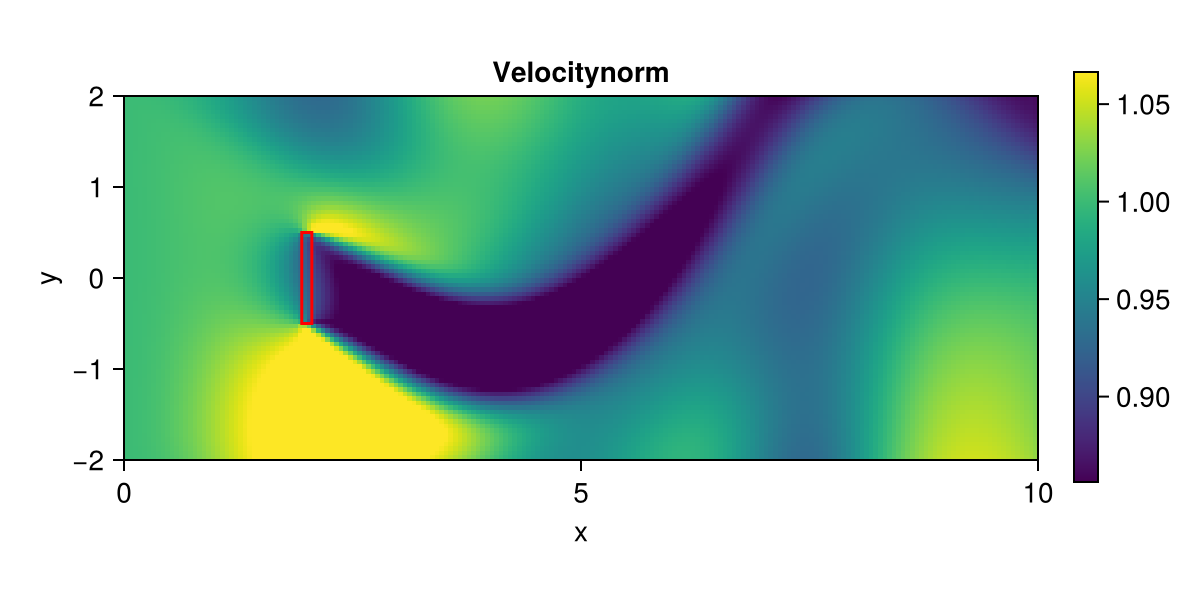

Plot vorticity

fig = fieldplot(state; setup, size = (600, 300), fieldname = :vorticity)
lines!(box...; color = :red)
fig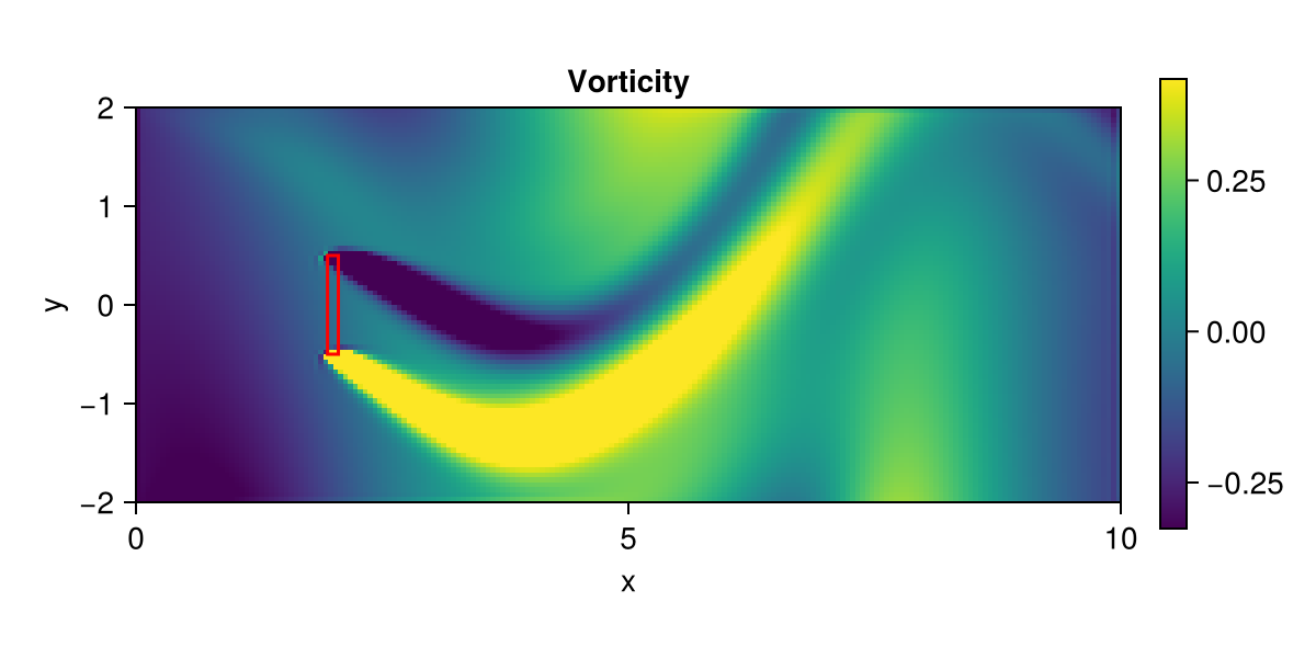

Copy-pasteable code

Below is the full code for this example stripped of comments and output.

using WGLMakie
using IncompressibleNavierStokes

n = 40
x = LinRange(0.0, 10.0, 5n + 1), LinRange(-2.0, 2.0, 2n + 1)
plotgrid(x...; figure = (; size = (600, 300)))

inflow(dim, x, y, t) = sinpi(sinpi(t / 6) / 6 + (dim == 1) / 2)
boundary_conditions =
    (; u = ((DirichletBC(inflow), PressureBC()), (PressureBC(), PressureBC())))

setup = Setup(; x, boundary_conditions);

xc, yc = 2.0, 0.0 # Disk center
D = 1.0           # Disk diameter
δ = 0.11          # Disk thickness
C = 0.2           # Thrust coefficient
c = C / (D * δ)   # Normalize
inside(x, y) = abs(x - xc) ≤ δ / 2 && abs(y - yc) ≤ D / 2
f(dim, x, y) = -c * (dim == 1) * inside(x, y)

function force!(f, state, t; setup, cache, viscosity)
    navierstokes!(f, state, t; setup, cache, viscosity)
    f.u .+= cache.bodyforce
end

IncompressibleNavierStokes.get_cache(::typeof(force!), setup) =
    (; bodyforce = velocityfield(setup, f; doproject = false))

u = velocityfield(setup, (dim, x, y) -> inflow(dim, x, y, 0.0));

state, outputs = solve_unsteady(;
    setup,
    force!,
    params = (; viscosity = 0.01),
    start = (; u),
    tlims = (0.0, 12e0),
    processors = (
        rtp = realtimeplotter(; setup, size = (600, 300), nupdate = 5),
        log = timelogger(; nupdate = 100),
    ),
);

box = (
    [xc - δ / 2, xc - δ / 2, xc + δ / 2, xc + δ / 2, xc - δ / 2],
    [yc + D / 2, yc - D / 2, yc - D / 2, yc + D / 2, yc + D / 2],
)

fig = fieldplot(state; setup, size = (600, 300), fieldname = :velocitynorm)
lines!(box...; color = :red)
fig

fig = fieldplot(state; setup, size = (600, 300), fieldname = :vorticity)
lines!(box...; color = :red)
fig

---

This page was generated using Literate.jl.