Decaying Homogeneous Isotropic Turbulence - 2D
In this example we consider decaying homogeneous isotropic turbulence, similar to the cases considered in [1] and [2]. The initial velocity field is created randomly, but with a specific energy spectrum. Due to viscous dissipation, the turbulent features eventually group to form larger visible eddies.
julia
using CairoMakie
using IncompressibleNavierStokes
Output directory
julia
outdir = joinpath(@__DIR__, "output", "DecayingTurbulence2D")"/home/runner/work/IncompressibleNavierStokes.jl/IncompressibleNavierStokes.jl/docs/build/examples/generated/output/DecayingTurbulence2D"Floating point precision
julia
T = Float64Float64Array type
julia
ArrayType = Array
# using CUDA; ArrayType = CuArray
# using AMDGPU; ArrayType = ROCArray
# using oneAPI; ArrayType = oneArray
# using Metal; ArrayType = MtlArrayArrayViscosity model
julia
Re = T(10_000)10000.0A 2D grid is a Cartesian product of two vectors
julia
n = 256
lims = T(0), T(1)
x = LinRange(lims..., n + 1), LinRange(lims..., n + 1)
(LinRange{Float64}(0.0, 1.0, 257), LinRange{Float64}(0.0, 1.0, 257))Build setup and assemble operators
julia
setup = Setup(; x, Re, ArrayType);Create random initial conditions
julia
ustart = random_field(setup, T(0));Solve unsteady problem
julia
state, outputs = solve_unsteady(;
    setup,
    ustart,
    tlims = (T(0), T(1)),
    Δt = T(1e-3),
    processors = (
        rtp = realtimeplotter(; setup, nupdate = 10),
        ehist = realtimeplotter(;
            setup,
            plot = energy_history_plot,
            nupdate = 10,
            displayfig = false,
        ),
        espec = realtimeplotter(;
            setup,
            plot = energy_spectrum_plot,
            nupdate = 10,
            displayfig = false,
        ),
        # anim = animator(; setup, path = joinpath(outdir, "solution.mp4"), nupdate = 10),
        # vtk = vtk_writer(; setup, nupdate = 10, dir = outdir, filename = "solution"),
        # field = fieldsaver(; setup, nupdate = 10),
        log = timelogger(; nupdate = 100),
    ),
);
[ Info: Iteration 100 t = 0.1 Δt = 0.001 umax = 3.54825
[ Info: Iteration 200 t = 0.2 Δt = 0.001 umax = 3.88136
[ Info: Iteration 300 t = 0.3 Δt = 0.001 umax = 3.45713
[ Info: Iteration 400 t = 0.4 Δt = 0.001 umax = 3.2843
[ Info: Iteration 500 t = 0.5 Δt = 0.001 umax = 2.8875
[ Info: Iteration 600 t = 0.6 Δt = 0.001 umax = 3.6285
[ Info: Iteration 700 t = 0.7 Δt = 0.001 umax = 2.75831
[ Info: Iteration 800 t = 0.8 Δt = 0.001 umax = 2.95543
[ Info: Iteration 900 t = 0.9 Δt = 0.001 umax = 2.7444
[ Info: Iteration 1000 t = 1 Δt = 0.001 umax = 2.76907Post-process
We may visualize or export the computed fields
Export to VTK
julia
save_vtk(state; setup, filename = joinpath(outdir, "solution"))1-element Vector{String}:
"/home/runner/work/Incompressibl" ⋯ 86 bytes ⋯ "cayingTurbulence2D/solution.vtr"Energy history
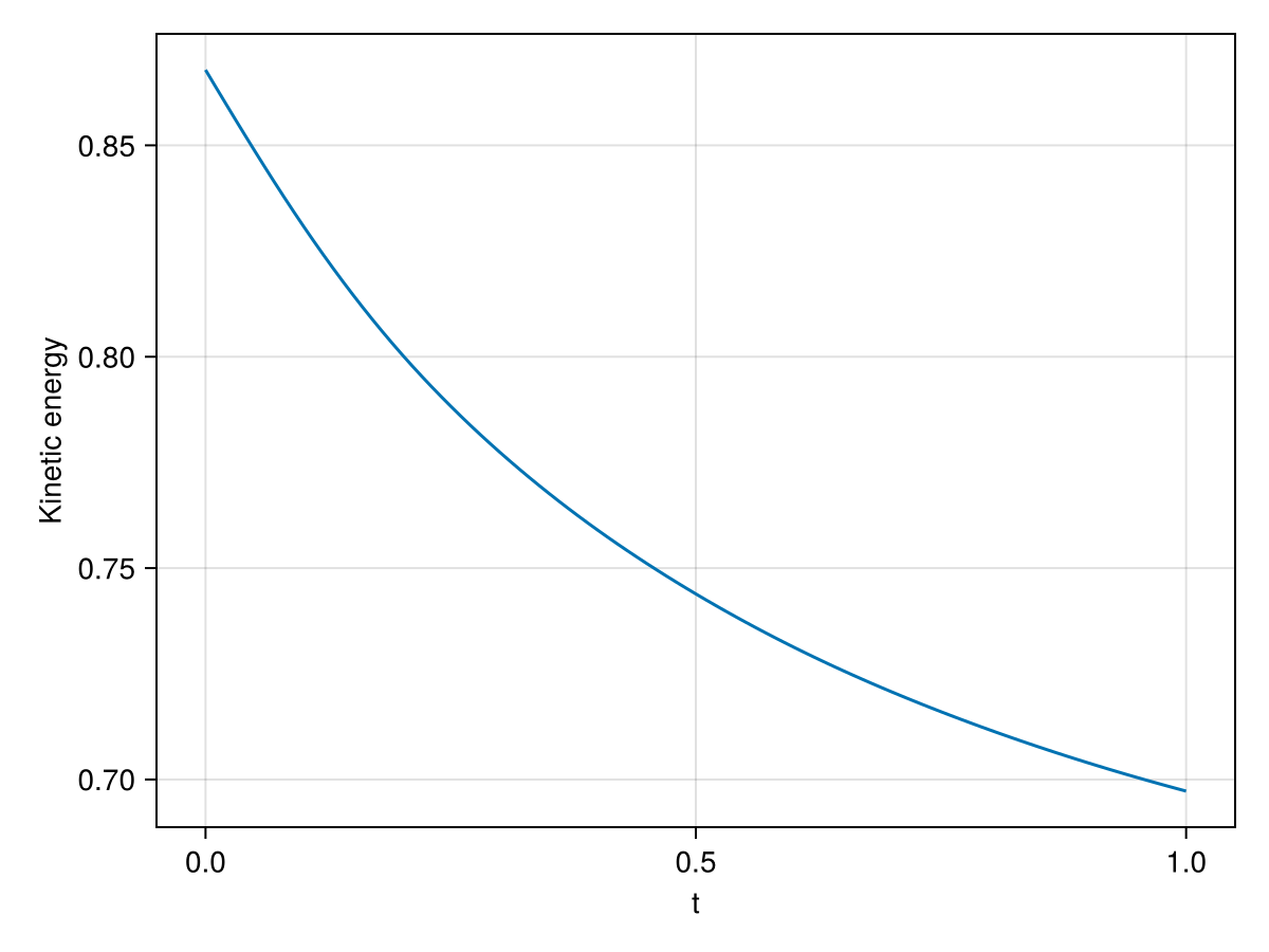
julia
outputs.ehist
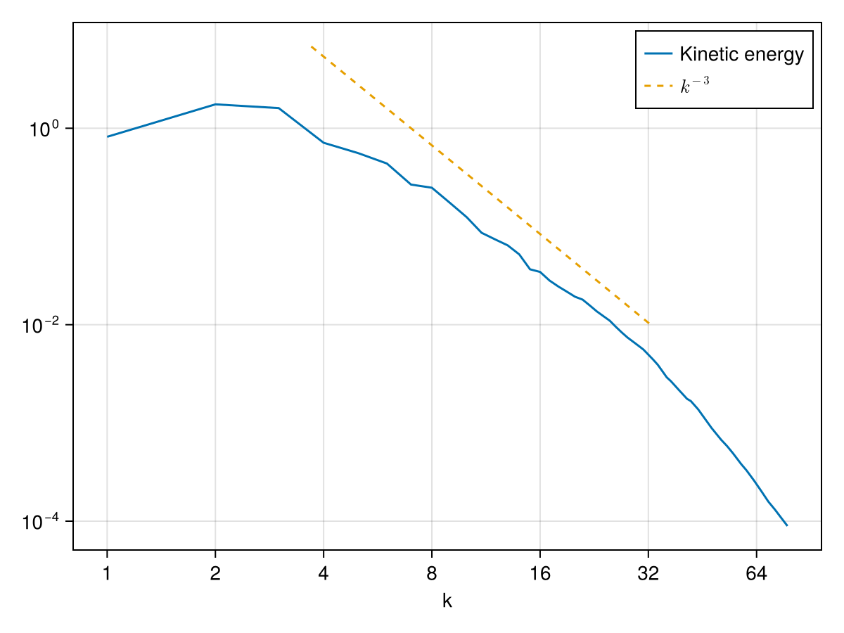
Energy spectrum
julia
outputs.espec
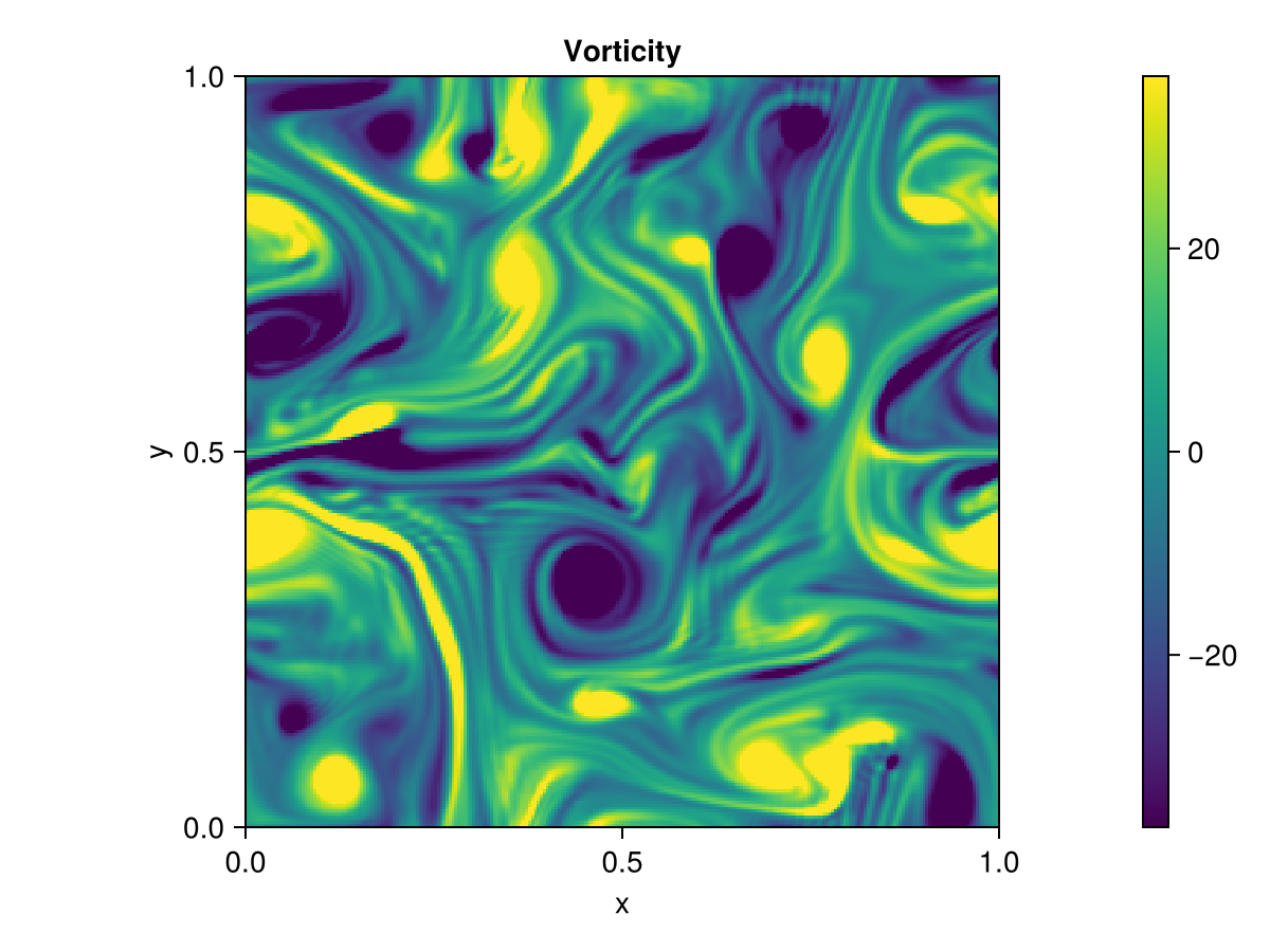
Plot field
julia
fieldplot(state; setup)
This page was generated using Literate.jl.