Steady lid-driven cavity (2D)

In the unsteady lid-driven cavity example, the flow approaches a steady state by marching in time. Here we instead solve directly for the steady state with a matrix-free Newton-Krylov method, using NonlinearSolve.jl.

Formulation

A discrete velocity field $u$ is a steady state if it is divergence-free and the momentum force $F(u)$ (convection and diffusion) is exactly balanced by a pressure gradient. Both conditions can be expressed with the pressure projection $\mathrm{\Pi }$ (which makes a field divergence-free by subtracting a pressure gradient): $u$ is steady if, and only if,

$$r(u)=u-\mathrm{\Pi }(u+\mathrm{\Delta }tF(u))=0,$$

i.e. if $u$ is a fixed point of a projection time step. The residual $r$ splits into a divergence-free part $-\mathrm{\Delta }t\mathrm{\Pi }F(u)$ and a pressure-gradient part $u-\mathrm{\Pi }u$, so $r=0$ enforces both $\mathrm{\Pi }F(u)=0$ and $\mathrm{\nabla }\cdot u=0$ at once. The pseudo-time step $\mathrm{\Delta }t>0$ does not change the solution; it only sets the relative weight of the two parts.

We solve $r(u)=0$ with Newton's method. The Jacobian is never assembled: GMRES only needs Jacobian-vector products, which NonlinearSolve.jl approximates with finite differences of $r$. Each residual evaluation is one right-hand side evaluation and one Poisson solve.

using CairoMakie
using IncompressibleNavierStokes
import IncompressibleNavierStokes as INS
using LinearAlgebra
using NonlinearSolve

Problem setup

The classic benchmark: a unit box with a lid moving at unit velocity, and a grid refined near the walls. The Reynolds number is set through the viscosity, $Re=1/\nu$.

boundary_conditions = (; u = (
    # x left, x right
    (DirichletBC(), DirichletBC()),

    # y bottom, y top
    (DirichletBC(), DirichletBC((1.0, 0.0))),
))

n = 64
ax = tanh_grid(0.0, 1.0, n)
setup = Setup(; x = (ax, ax), boundary_conditions);
psolver = default_psolver(setup);

Residual

The unknowns of the nonlinear problem are the interior velocity components (the degrees of freedom), gathered into a flat vector. Ghost volumes and boundary faces are excluded: they are determined by the boundary conditions, and keeping them as unknowns would make the Jacobian singular.

"Gather velocity DOFs (interior points) into a flat vector."
function field2dofs!(v, u, setup)
    (; dimension, Iu) = setup
    i = 0
    for α = 1:dimension()
        nα = length(Iu[α])
        copyto!(view(v, (i+1):(i+nα)), view(u, Iu[α], α))
        i += nα
    end
    v
end

"Scatter a flat DOF vector into a full velocity field (ghosts untouched)."
function dofs2field!(u, v, setup)
    (; dimension, Iu) = setup
    i = 0
    for α = 1:dimension()
        nα = length(Iu[α])
        copyto!(view(u, Iu[α], α), view(v, (i+1):(i+nα)))
        i += nα
    end
    u
end

Main.dofs2field!

The residual $r(u)=u-\mathrm{\Pi }(u+\mathrm{\Delta }tF(u))$ maps DOF vector to DOF vector. All fields are preallocated in the parameter tuple, so one evaluation costs one force evaluation and one Poisson solve.

function steady_residual!(r, v, prm)
    (; ucache, fcache, pcache, setup, psolver, viscosity, Δt) = prm
    T = eltype(v)
    u = dofs2field!(ucache, v, setup)
    INS.apply_bc_u!(u, zero(T), setup)
    fill!(fcache, 0)
    INS.convectiondiffusion!(fcache, u, setup, viscosity)
    @. fcache = u + Δt * fcache
    INS.apply_bc_u!(fcache, zero(T), setup)
    INS.project!(fcache, setup; psolver, p = pcache)
    field2dofs!(r, fcache, setup)
    @. r = v - r
    r
end

steady_residual! (generic function with 1 method)

Newton-Krylov solver

Newton's method with backtracking line search; the linear systems are solved matrix-free with GMRES. AutoFiniteDiff makes NonlinearSolve approximate Jacobian-vector products with finite differences of the (mutating, hence not dual-number-compatible) residual.

function solve_steady(v0, viscosity; setup, psolver, Δt = 1.0, abstol = 1e-10)
    prm = (;
        ucache = vectorfield(setup),
        fcache = vectorfield(setup),
        pcache = scalarfield(setup),
        setup,
        psolver,
        viscosity,
        Δt,
    )
    prob = NonlinearProblem(NonlinearFunction(steady_residual!), copy(v0), prm)
    alg = NewtonRaphson(;
        linsolve = KrylovJL_GMRES(),
        autodiff = AutoFiniteDiff(),
        jvp_autodiff = AutoFiniteDiff(),
        linesearch = BackTracking(),
    )
    sol = solve(prob, alg; abstol, maxiters = 50)
    @info "Re = $(1 / viscosity)" sol.retcode sol.stats.nsteps norm(sol.resid)
    sol.u
end

solve_steady (generic function with 1 method)

Initial guess and continuation

Newton's method needs a reasonable initial guess. Starting impulsively from rest diverges, so we march in time for a couple of time units first (a "burn-in"), and then let Newton polish the result to machine precision.

ustart = velocityfield(setup, (dim, x, y) -> zero(x));
state, _ = solve_unsteady(;
    setup,
    start = (; u = ustart),
    tlims = (0.0, 2.0),
    params = (; viscosity = 1e-2),
    psolver,
);
v0 = field2dofs!(zeros(sum(length, setup.Iu)), state.u, setup);

This suffices for $Re=100$:

v100 = solve_steady(v0, 1e-2; setup, psolver);

┌ Info: Re = 100.0
│   sol.retcode = ReturnCode.Success = 1
│   sol.stats.nsteps = 4
└   norm(sol.resid) = 9.63615044928241e-11

For higher Reynolds numbers the basin of attraction shrinks, but each steady state is an excellent initial guess for the next Reynolds number. Such a continuation takes us to $Re=1000$ in two more solves, without any further time stepping:

v400 = solve_steady(v100, 2.5e-3; setup, psolver);
v1000 = solve_steady(v400, 1e-3; setup, psolver);

┌ Info: Re = 400.0
│   sol.retcode = ReturnCode.Success = 1
│   sol.stats.nsteps = 5
└   norm(sol.resid) = 1.004462299134325e-10
┌ Info: Re = 1000.0
│   sol.retcode = ReturnCode.Success = 1
│   sol.stats.nsteps = 7
└   norm(sol.resid) = 9.953039461893647e-11

Note that time-marching to the $Re=1000$ steady state would require hundreds of time units (tens of thousands of time steps), while Newton converges in a handful of iterations per Reynolds number.

Validation

Ghia, Ghia, and Shin [4] provide reference values for the horizontal velocity along the vertical centerline of the cavity.

yghia = [
    0.0000,
    0.0547,
    0.0625,
    0.0703,
    0.1016,
    0.1719,
    0.2813,
    0.4531,
    0.5000,
    0.6172,
    0.7344,
    0.8516,
    0.9531,
    0.9609,
    0.9688,
    0.9766,
    1.0000,
]
ughia = (;
    Re100 = [
        0.0000,
        -0.03717,
        -0.04192,
        -0.04775,
        -0.06434,
        -0.10150,
        -0.15662,
        -0.21090,
        -0.20581,
        -0.13641,
        0.00332,
        0.23151,
        0.68717,
        0.73722,
        0.78871,
        0.84123,
        1.0000,
    ],
    Re1000 = [
        0.0000,
        -0.18109,
        -0.20196,
        -0.22220,
        -0.29730,
        -0.38289,
        -0.27805,
        -0.10648,
        -0.06080,
        0.05702,
        0.18719,
        0.33304,
        0.46604,
        0.51117,
        0.57492,
        0.65928,
        1.0000,
    ],
);

The first velocity component lives on the volume faces, so with an even number of volumes there is a line of points exactly on the centerline $x=1/2$.

function centerline(v)
    u = INS.apply_bc_u!(dofs2field!(vectorfield(setup), v, setup), 0.0, setup)
    (; xu) = setup
    i = findfirst(≈(0.5), xu[1][1])
    y = xu[1][2][2:(end-1)]
    (y, u[i, 2:(end-1), 1])
end

fig = Figure()
axis = Axis(fig[1, 1]; xlabel = "u₁(0.5, y)", ylabel = "y")
for (v, Re, color) in ((v100, :Re100, 1), (v1000, :Re1000, 2))
    y, uline = centerline(v)
    lines!(axis, uline, y; color = Cycled(color), label = "Re = $(string(Re)[3:end])")
    scatter!(axis, ughia[Re], yghia; color = Cycled(color))
end
axislegend(axis; position = :rb)
fig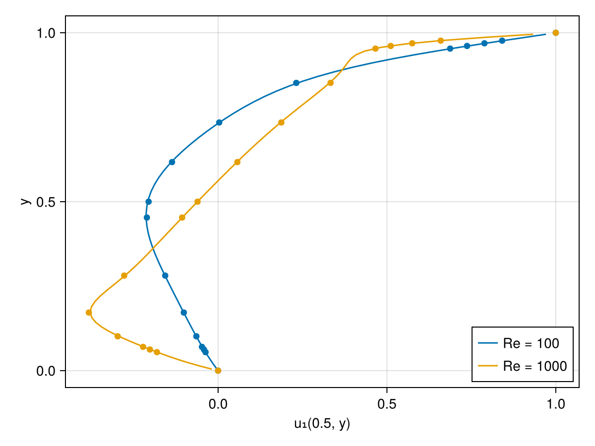

The computed profiles (lines) pass through the reference values (dots).

Plot fields

The $Re=1000$ steady state, with the classic secondary vortices in the bottom corners:

u = INS.apply_bc_u!(dofs2field!(vectorfield(setup), v1000, setup), 0.0, setup)
fieldplot((; u, t = 0.0); setup, fieldname = :velocitynorm)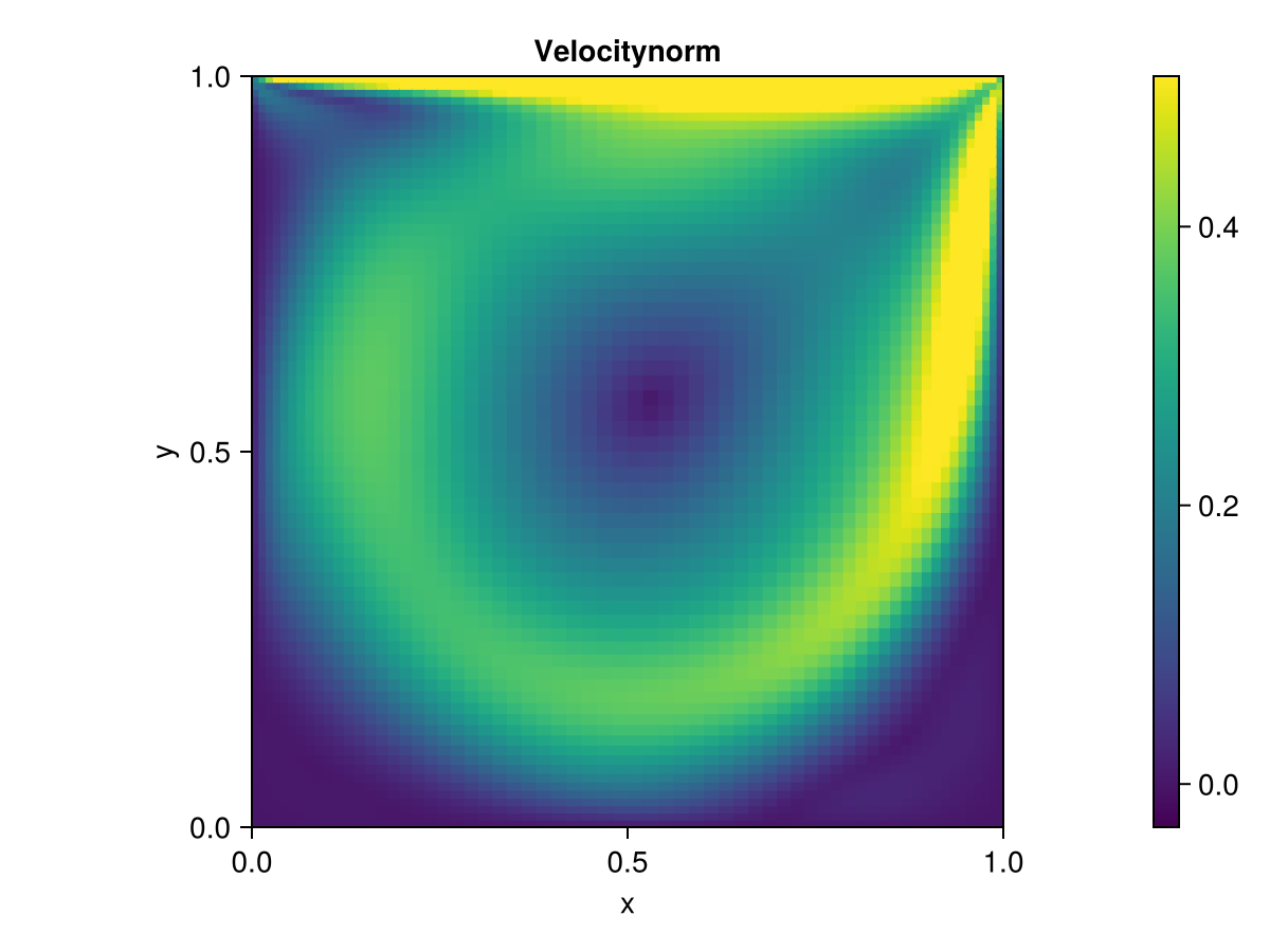

fieldplot((; u, t = 0.0); setup, fieldname = :vorticity)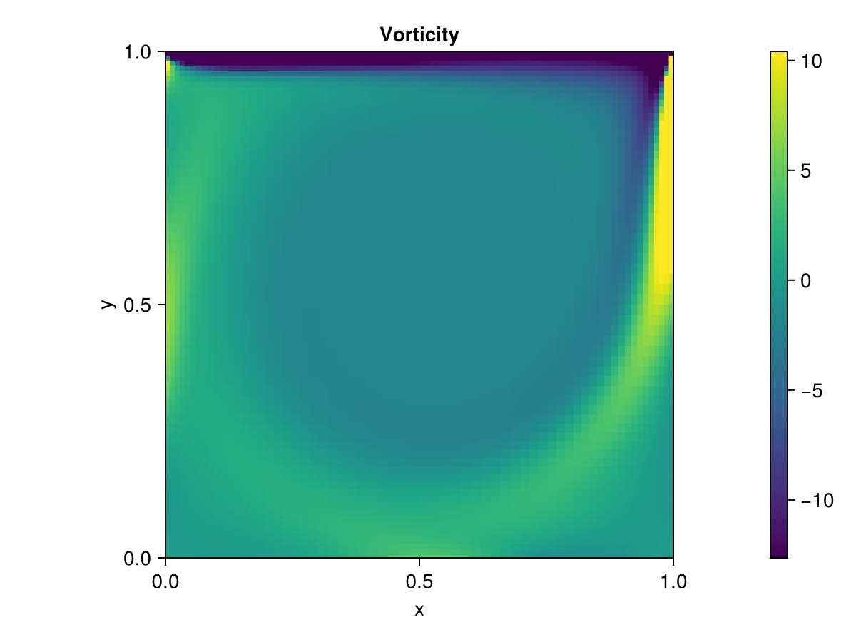

Remarks

• The GMRES iterations are not preconditioned, and their number grows with the Reynolds number and the grid resolution. For larger problems, a preconditioner (e.g. based on the diffusion operator, see diffusion_mat) becomes necessary.

• Newton's method converges to unstable steady states just as happily as to stable ones (unlike time marching, which only finds stable ones). This is a feature: together with continuation, it can track solution branches beyond the point where the steady cavity flow loses stability (around $Re\approx 8000$).

Copy-pasteable code

Below is the full code for this example stripped of comments and output.

using WGLMakie
using IncompressibleNavierStokes
import IncompressibleNavierStokes as INS
using LinearAlgebra
using NonlinearSolve

boundary_conditions = (; u = (
    # x left, x right
    (DirichletBC(), DirichletBC()),

    # y bottom, y top
    (DirichletBC(), DirichletBC((1.0, 0.0))),
))

n = 64
ax = tanh_grid(0.0, 1.0, n)
setup = Setup(; x = (ax, ax), boundary_conditions);
psolver = default_psolver(setup);

"Gather velocity DOFs (interior points) into a flat vector."
function field2dofs!(v, u, setup)
    (; dimension, Iu) = setup
    i = 0
    for α = 1:dimension()
        nα = length(Iu[α])
        copyto!(view(v, (i+1):(i+nα)), view(u, Iu[α], α))
        i += nα
    end
    v
end

"Scatter a flat DOF vector into a full velocity field (ghosts untouched)."
function dofs2field!(u, v, setup)
    (; dimension, Iu) = setup
    i = 0
    for α = 1:dimension()
        nα = length(Iu[α])
        copyto!(view(u, Iu[α], α), view(v, (i+1):(i+nα)))
        i += nα
    end
    u
end

function steady_residual!(r, v, prm)
    (; ucache, fcache, pcache, setup, psolver, viscosity, Δt) = prm
    T = eltype(v)
    u = dofs2field!(ucache, v, setup)
    INS.apply_bc_u!(u, zero(T), setup)
    fill!(fcache, 0)
    INS.convectiondiffusion!(fcache, u, setup, viscosity)
    @. fcache = u + Δt * fcache
    INS.apply_bc_u!(fcache, zero(T), setup)
    INS.project!(fcache, setup; psolver, p = pcache)
    field2dofs!(r, fcache, setup)
    @. r = v - r
    r
end

function solve_steady(v0, viscosity; setup, psolver, Δt = 1.0, abstol = 1e-10)
    prm = (;
        ucache = vectorfield(setup),
        fcache = vectorfield(setup),
        pcache = scalarfield(setup),
        setup,
        psolver,
        viscosity,
        Δt,
    )
    prob = NonlinearProblem(NonlinearFunction(steady_residual!), copy(v0), prm)
    alg = NewtonRaphson(;
        linsolve = KrylovJL_GMRES(),
        autodiff = AutoFiniteDiff(),
        jvp_autodiff = AutoFiniteDiff(),
        linesearch = BackTracking(),
    )
    sol = solve(prob, alg; abstol, maxiters = 50)
    @info "Re = $(1 / viscosity)" sol.retcode sol.stats.nsteps norm(sol.resid)
    sol.u
end

ustart = velocityfield(setup, (dim, x, y) -> zero(x));
state, _ = solve_unsteady(;
    setup,
    start = (; u = ustart),
    tlims = (0.0, 2.0),
    params = (; viscosity = 1e-2),
    psolver,
);
v0 = field2dofs!(zeros(sum(length, setup.Iu)), state.u, setup);

v100 = solve_steady(v0, 1e-2; setup, psolver);

v400 = solve_steady(v100, 2.5e-3; setup, psolver);
v1000 = solve_steady(v400, 1e-3; setup, psolver);

yghia = [
    0.0000,
    0.0547,
    0.0625,
    0.0703,
    0.1016,
    0.1719,
    0.2813,
    0.4531,
    0.5000,
    0.6172,
    0.7344,
    0.8516,
    0.9531,
    0.9609,
    0.9688,
    0.9766,
    1.0000,
]
ughia = (;
    Re100 = [
        0.0000,
        -0.03717,
        -0.04192,
        -0.04775,
        -0.06434,
        -0.10150,
        -0.15662,
        -0.21090,
        -0.20581,
        -0.13641,
        0.00332,
        0.23151,
        0.68717,
        0.73722,
        0.78871,
        0.84123,
        1.0000,
    ],
    Re1000 = [
        0.0000,
        -0.18109,
        -0.20196,
        -0.22220,
        -0.29730,
        -0.38289,
        -0.27805,
        -0.10648,
        -0.06080,
        0.05702,
        0.18719,
        0.33304,
        0.46604,
        0.51117,
        0.57492,
        0.65928,
        1.0000,
    ],
);

function centerline(v)
    u = INS.apply_bc_u!(dofs2field!(vectorfield(setup), v, setup), 0.0, setup)
    (; xu) = setup
    i = findfirst(≈(0.5), xu[1][1])
    y = xu[1][2][2:(end-1)]
    (y, u[i, 2:(end-1), 1])
end

fig = Figure()
axis = Axis(fig[1, 1]; xlabel = "u₁(0.5, y)", ylabel = "y")
for (v, Re, color) in ((v100, :Re100, 1), (v1000, :Re1000, 2))
    y, uline = centerline(v)
    lines!(axis, uline, y; color = Cycled(color), label = "Re = $(string(Re)[3:end])")
    scatter!(axis, ughia[Re], yghia; color = Cycled(color))
end
axislegend(axis; position = :rb)
fig

u = INS.apply_bc_u!(dofs2field!(vectorfield(setup), v1000, setup), 0.0, setup)
fieldplot((; u, t = 0.0); setup, fieldname = :velocitynorm)

fieldplot((; u, t = 0.0); setup, fieldname = :vorticity)

---

This page was generated using Literate.jl.