Spatial and temporal discretization

This page describes the discretization used in the solver, in the same notation as the code. The domain is discretized on a staggered Cartesian grid as proposed by Harlow and Welch [5], and the equations are stepped in time with explicit Runge-Kutta methods [6].

Staggered grid

The rectangular domain $\mathrm{\Omega }=\prod _{\alpha =1}^d[a_{\alpha },b_{\alpha }]$ is partitioned into finite volumes

$${\mathrm{\Omega }}_I=\prod _{\alpha =1}^d[x_{I_{\alpha }-1}^{\alpha },x_{I_{\alpha }}^{\alpha }],$$

indexed by the Cartesian index $I=(I_1,\dots ,I_d)$. The Cartesian index lets us write dimension-agnostic expressions such as $u_I$ instead of $u_{ij}$ in 2D or $u_{ijk}$ in 3D, and the code uses the same convention (u[I] instead of u[i, j] or u[i, j, k]). The $\alpha$-th unit vector is denoted $e_{\alpha }$, e.g. $I+e_2=(I_1,I_2+1,I_3)$ in 3D. The grid is defined by the volume boundary coordinates $x_i^{\alpha }$ passed to Setup (the vectors x[α]), from which the volume widths ${\mathrm{\Delta }}_i^{\alpha }=x_i^{\alpha }-x_{i-1}^{\alpha }$ (the vectors Δ[α]) follow. The grid does not need to be uniform.

The unknowns are staggered:

• The pressure $p_I$ is defined in the volume center.

• The velocity component $u_I^{\alpha }$ is defined on the right face of volume $I$ in direction $\alpha$, i.e. on the boundary between ${\mathrm{\Omega }}_I$ and ${\mathrm{\Omega }}_{I+e_{\alpha }}$. In the code, all components are stored in one array with the component as the last index: u[I, α].

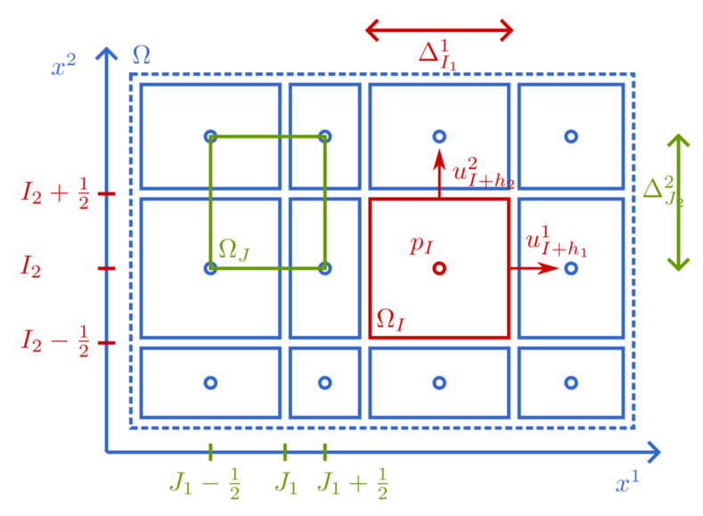
In addition to the interior volumes, all fields carry one layer of ghost volumes on each boundary. The ghost values are filled by apply_bc_u! and apply_bc_p! such that the interior finite-volume stencils automatically account for the boundary conditions (Dirichlet, periodic, symmetric, or pressure). This is why the field arrays have size N while the degrees of freedom are indexed by Ip and Iu.

Mass equation

Integrating the mass equation over the pressure volume ${\mathrm{\Omega }}_I$ and approximating the face integrals with the mid-point rule gives the discrete divergence-free constraint

$$\sum _{\alpha =1}^d\frac{u_I^{\alpha }-u_{I-e_{\alpha }}^{\alpha }}{{\mathrm{\Delta }}_{I_{\alpha }}^{\alpha }}=0,$$

a backward difference of the face velocities surrounding the pressure volume. This is the divergence operator. Since we divided by the volume size, the discrete equation resembles the continuous one $\mathrm{\nabla }\cdot u=0$.

Momentum equations

The momentum equation for $u^{\alpha }$ is integrated over the shifted volume centered on the $\alpha$-face. Approximating the face integrals with the mid-point rule and the diffusive fluxes with central differences gives

$$\frac{\mathrm{d}}{\mathrm{d}t}{u}_I^{\alpha }=-\sum _{\beta =1}^d({\delta }_{\beta }(u^{\alpha }{u}^{\beta }){)}_I+\nu \sum _{\beta =1}^d({\delta }_{\beta }{\delta }_{\beta }{u}^{\alpha }{)}_I+f_I^{\alpha }-({\delta }_{\alpha }p{)}_I,$$

where ${\delta }_{\beta }$ denotes the central difference in direction $\beta$ at the position in question. The pressure gradient is a forward difference of the two pressure values adjacent to the $\alpha$-face (pressuregradient). In the convective term, the two velocity components in the product $u^{\alpha }{u}^{\beta }$ are not stored at the required position; they are obtained by averaging with weights $1/2$ for the $\alpha$-component and linear interpolation for the $\beta$-component. This particular choice preserves the skew-symmetry of the convection operator on uniform grids, such that convection neither creates nor destroys kinetic energy [7]. Convection and diffusion are implemented together in the right-hand side force navierstokes!, with convection and diffusion as separate differentiable operators.

All operators come in two variants: a fast mutating one (e.g. divergence!) and a differentiable non-mutating one (e.g. divergence). See Operators and Differentiating code.

Discrete pressure Poisson equation

Instead of discretizing the continuous pressure Poisson equation, we require that the discrete velocity field stays divergence free. Let $M$ denote the discrete divergence, $G$ the discrete pressure gradient, $W$ the diagonal matrix of pressure volume sizes, and $F(u)$ all discrete forces except the pressure gradient. Applying $M$ to the discrete momentum equations and requiring $\frac{\mathrm{d}}{\mathrm{d}t}Mu=0$ yields

$$Lp=WMF(u),$$

where $L=WMG$ is a symmetric positive semi-definite discrete Laplacian. This equation is solved by the pressure solvers (poisson, see Pressure solvers). Subtracting the resulting pressure gradient projects a velocity field onto the space of discretely divergence-free fields; this is the project operator. Without pressure boundary conditions $L$ has a zero eigenvalue and the pressure is determined up to a constant, which we set to zero.

Sparse matrix representations of $M$, $G$, $L$, $W$, and the boundary condition kernels are available, see Sparse matrices.

Time discretization

The spatially discretized system is a differential-algebraic system: an ODE for the velocity subject to the algebraic divergence-free constraint. It is stepped in time with explicit Runge-Kutta methods, where each stage velocity is made divergence free by a pressure projection. This retains the accuracy of the underlying Runge-Kutta method for the velocity; see Sanderse and Koren [6] for an analysis.

Given the state $u^n$ at time $t^n$, a stage $i$ of an explicit method with tableau $(A,b,c)$ computes

$$u_i=\mathrm{\Pi }(u^n+\mathrm{\Delta }t\sum _{j<i}{a}_{ij}F(u_j,t_j)),$$

where $\mathrm{\Pi }$ is the pressure projection, and the next step $u^{n+1}$ follows analogously with weights $b_j$. The default method is LMWray3, a low-storage third-order method of Wray [8] that only needs three vector fields of storage. A large collection of tableaus is available in RKMethods.

The time step can be fixed (Δt) or chosen adaptively from a CFL condition based on the convective and diffusive stability limits (Δt = nothing in solve_unsteady, the default).