Getting Started

To install IncompressibleNavierStokes, open up a Julia-REPL, type ] to get into Pkg-mode, and type:

add IncompressibleNavierStokes

which will install the package and all dependencies to your local environment. Note that IncompressibleNavierStokes requires Julia version 1.10 or above.

A first simulation

The following code simulates decaying turbulence in a periodic 2D box and plots the resulting vorticity field:

using IncompressibleNavierStokes
using CairoMakie

# Discretize the domain [0, 1]² into 128 × 128 finite volumes
n = 128
ax = range(0.0, 1.0, n + 1)
setup = Setup(;
    x = (ax, ax),
    boundary_conditions = (;
        u = ((PeriodicBC(), PeriodicBC()), (PeriodicBC(), PeriodicBC())),
    ),
)

# Random initial velocity field with a prescribed energy spectrum
u = random_field(setup)

# Solve the unsteady problem from t = 0 to t = 1
state, outputs = solve_unsteady(;
    setup,
    start = (; u),
    tlims = (0.0, 1.0),
    params = (; viscosity = 1e-3),
)

# Plot the vorticity of the final state
fieldplot(state; setup, fieldname = :vorticity)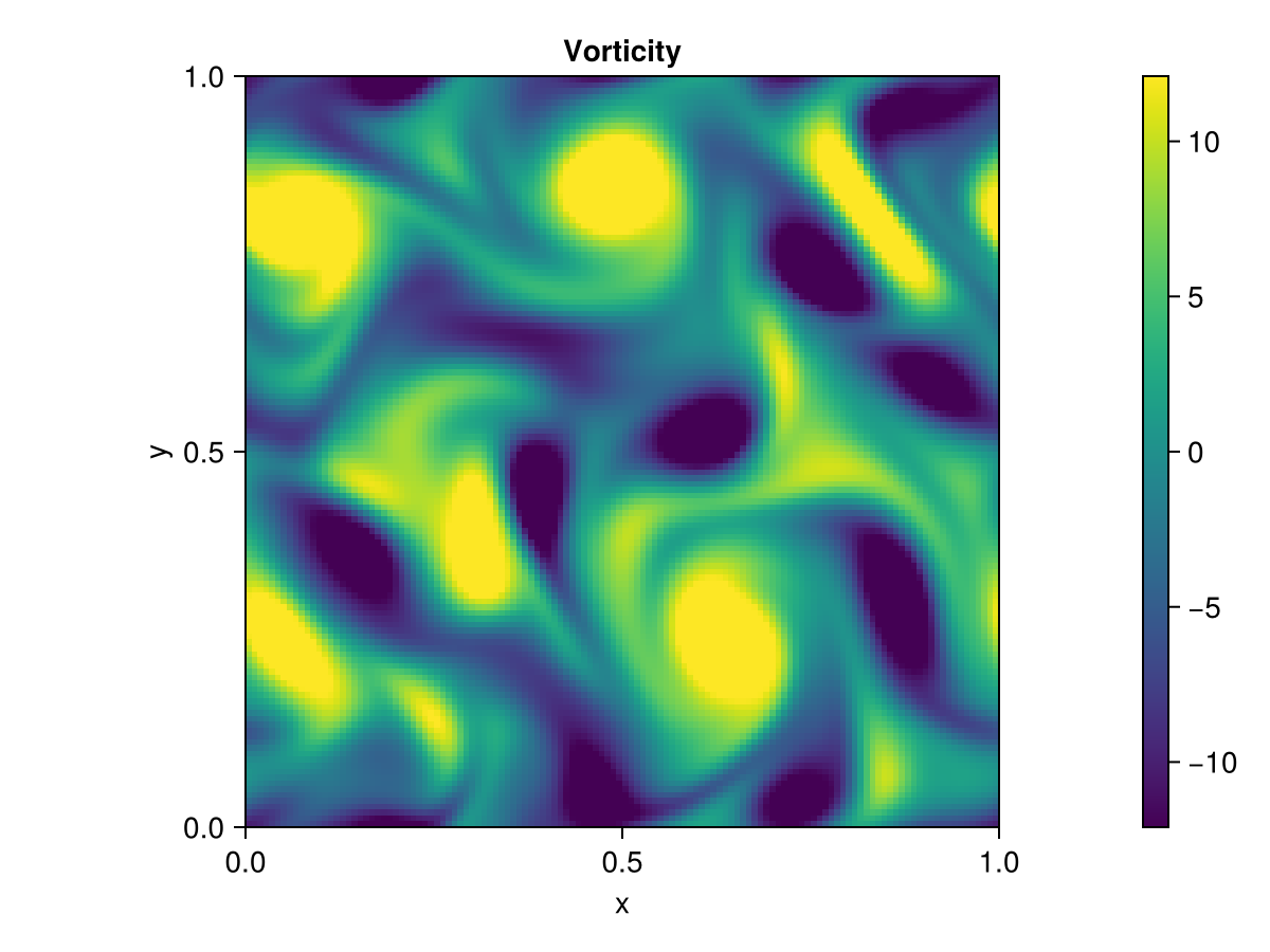

The building blocks appearing here:

• Setup defines the grid and boundary conditions — see Problem setup.

• random_field creates a divergence-free initial condition — see initializers.

• solve_unsteady steps the state through time; physical parameters like the viscosity are passed in params — see Solving unsteady problems.

• fieldplot and friends become available when a Makie backend is loaded — see Postprocessing.

Where to go next

• The examples gallery contains commented simulations of many flow configurations (cavities, actuator disks, channels, Rayleigh-Bénard convection, ...), including GPU usage.

• The manual documents the equations, the discretization, and the API.