Decaying Homogeneous Isotropic Turbulence - 2D

In this example we consider decaying homogeneous isotropic turbulence, similar to the cases considered in [2] and [3]. The initial velocity field is created randomly, but with a specific energy spectrum. Due to viscous dissipation, the turbulent features eventually group to form larger visible eddies.

Packages

We just need IncompressibleNavierStokes and a Makie plotting backend.

using CairoMakie
using IncompressibleNavierStokes
# using CUDA

Setup

n = 256
ax = LinRange(0.0, 1.0, n + 1)
setup = Setup(;
    x = (ax, ax),
    boundary_conditions = (;
        u = ((PeriodicBC(), PeriodicBC()), (PeriodicBC(), PeriodicBC())),
    ),
    # backend = CUDABackend(),
)
u = random_field(setup, 0.0);

Solve unsteady problem

state, outputs = solve_unsteady(;
    setup,
    start = (; u),
    tlims = (0.0, 1.0),
    params = (; viscosity = 2.5e-4),
    processors = (
        rtp = realtimeplotter(; setup, nupdate = 10),
        ehist = realtimeplotter(;
            setup,
            plot = energy_history_plot,
            nupdate = 10,
            displayfig = false,
        ),
        espec = realtimeplotter(;
            setup,
            plot = energy_spectrum_plot,
            nupdate = 10,
            displayfig = false,
        ),
        log = timelogger(; nupdate = 100),
    ),
);

[ Info: t = 0.0995275	Δt = 0.0011	umax = 3.2	itertime = 0.025
[ Info: t = 0.20202	Δt = 0.0009	umax = 3.9	itertime = 0.01
[ Info: t = 0.310514	Δt = 0.0013	umax = 2.7	itertime = 0.0097
[ Info: t = 0.438775	Δt = 0.0012	umax = 3	itertime = 0.0089
[ Info: t = 0.566904	Δt = 0.0014	umax = 2.5	itertime = 0.0089
[ Info: t = 0.711702	Δt = 0.0013	umax = 2.7	itertime = 0.0089
[ Info: t = 0.833034	Δt = 0.0011	umax = 3.1	itertime = 0.0092
[ Info: t = 0.954732	Δt = 0.0014	umax = 2.5	itertime = 0.0089
[ Info: Finished after 831 time steps and 9.3 seconds

Post-process

We may visualize or export the computed fields

Energy history

outputs.ehist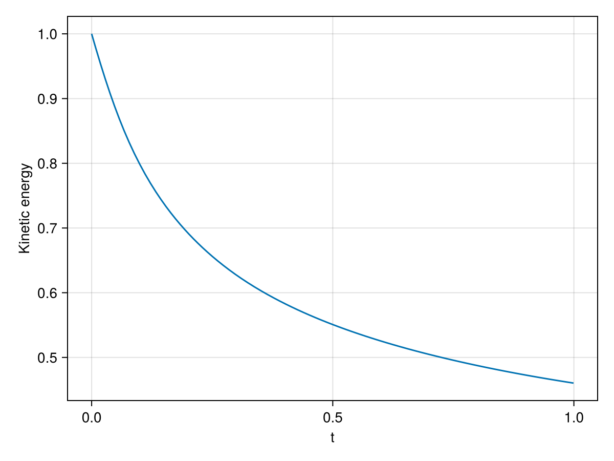

Energy spectrum

outputs.espec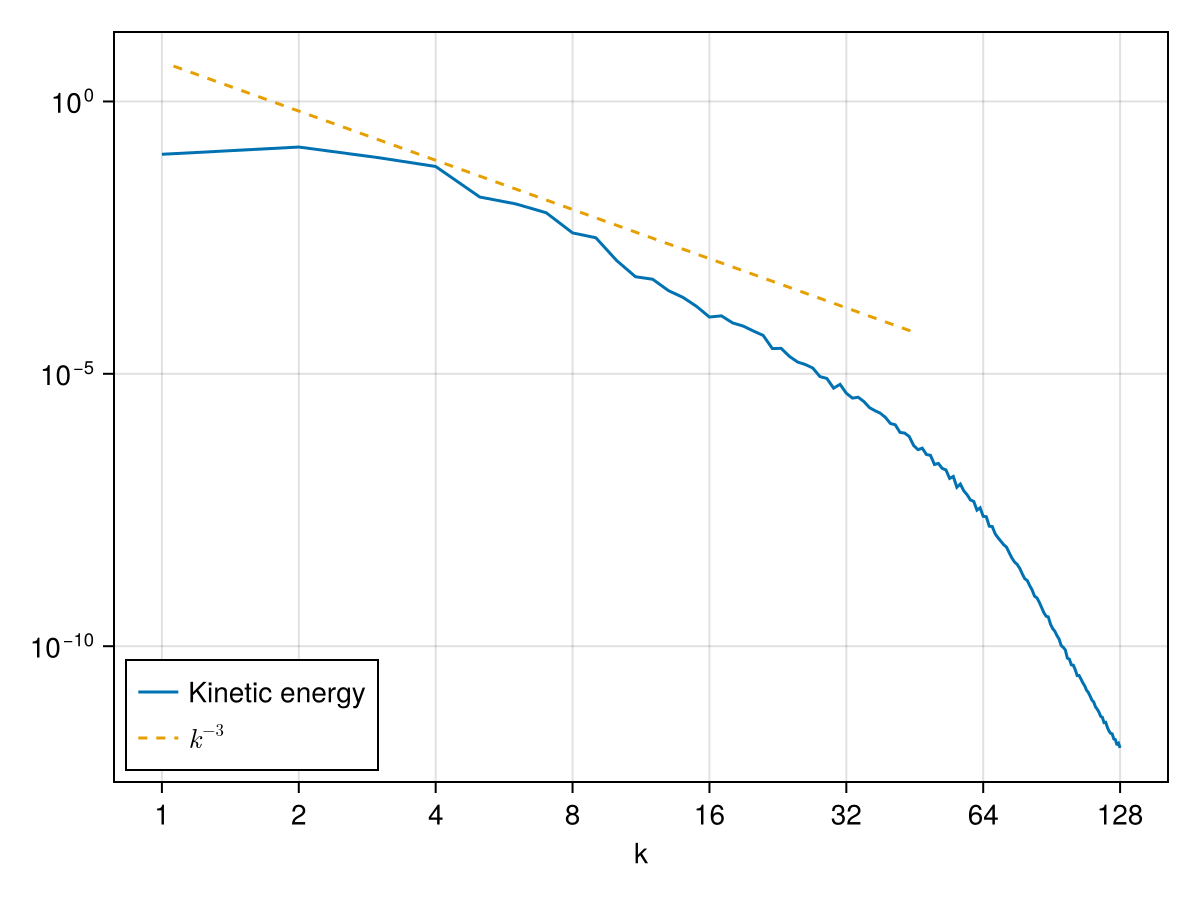

Plot field

fieldplot(state; setup)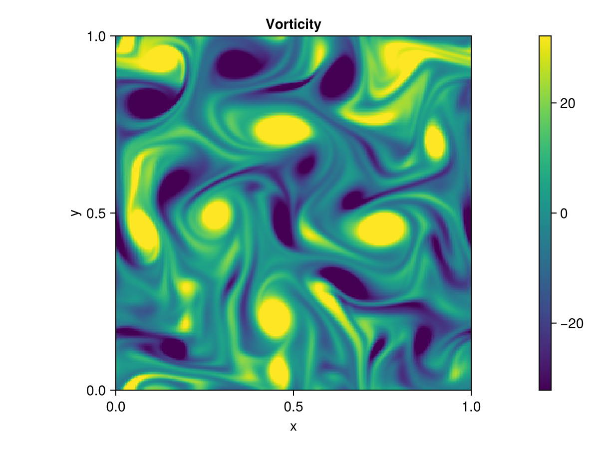

Copy-pasteable code

Below is the full code for this example stripped of comments and output.

using WGLMakie
using IncompressibleNavierStokes
# using CUDA

n = 256
ax = LinRange(0.0, 1.0, n + 1)
setup = Setup(;
    x = (ax, ax),
    boundary_conditions = (;
        u = ((PeriodicBC(), PeriodicBC()), (PeriodicBC(), PeriodicBC())),
    ),
    # backend = CUDABackend(),
)
u = random_field(setup, 0.0);

state, outputs = solve_unsteady(;
    setup,
    start = (; u),
    tlims = (0.0, 1.0),
    params = (; viscosity = 2.5e-4),
    processors = (
        rtp = realtimeplotter(; setup, nupdate = 10),
        ehist = realtimeplotter(;
            setup,
            plot = energy_history_plot,
            nupdate = 10,
            displayfig = false,
        ),
        espec = realtimeplotter(;
            setup,
            plot = energy_spectrum_plot,
            nupdate = 10,
            displayfig = false,
        ),
        log = timelogger(; nupdate = 100),
    ),
);

outputs.ehist

outputs.espec

fieldplot(state; setup)

---

This page was generated using Literate.jl.