(Draft) Writing a differentiable fluid solver in Julia

A journey from sparse matrices in MATLAB to differentiable GPU operators in Julia

IncompressibleNavierStokes.jl is a Julia package for solving the Incompressible Navier-Stokes equations given by

$$\begin{array}{rl}\mathrm{\nabla }\cdot u& =0,\\ \frac{\partial u}{\partial t}+\mathrm{\nabla }\cdot \left(u{u}^{\mathsf{T}}\right)& =\nu {\mathrm{\nabla }}^{2}u-\mathrm{\nabla }p,\end{array}$$

where $u$ is a 2D or 3D velocity field of a fluid, $p$ is the pressure, and $\nu$ is the viscosity. The equations are discretized on a staggered Cartesian grid^[1] as shown below:

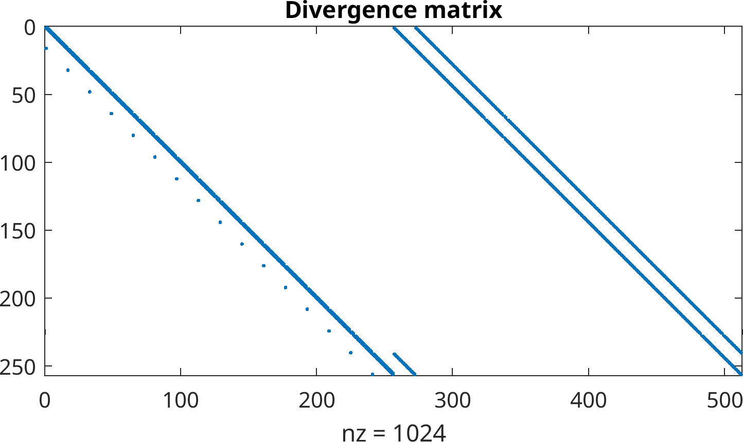
The velocity field is defined on the volume faces, and the pressure in the volume centers. The grid is Cartesian, but the volumes are allowed to have non-uniform sizes. This discretization is useful since the divergence constraint $\mathrm{\nabla }\cdot u=0$ is preserved discretely. In each volume, we impose

$$\frac{u_{\text{right}}-u_{\text{left}}}{\mathrm{\Delta }x}+\frac{u_{\text{top}}-u_{\text{bottom}}}{\mathrm{\Delta }y}=0.$$

Initial implementation: Sparse matrices

My PhD supervisor wrote an implementation a while back in MATLAB, using sparse matrices. The matrix equations equations take the following (integral) form:

$$\begin{array}{rl}Mu& =0,\\ \mathrm{\Omega }\frac{\mathrm{d}u}{\mathrm{d}t}+C(Au\odot Iu)& =\nu Du-Gp,\end{array}$$

where $M$ is a divergence matrix, $\mathrm{\Omega }$ is a diagonal matrix containing the volume of each cell, $C(Au\odot Iu)$ is an energy-preserving discretization of the convective term involving averaging and interpolation between volume faces, centers, and corners, $D$ is a diffusion matrix, $G=M^{\mathsf{T}}$ is a gradient matrix, and $u$ and $p$ are vectors containing all the velocity and pressure components.

Sparsity pattern of the divergence matrix on a 16x16 grid with a periodic domain. The left block discretizes d/dx, the right block d/dy. Each of the dots in the left block shows the periodic extension in the x-direction, before the y-index is incremented.

Matrices are very convenient to work with, since the code is identical to the mathematical matrix formulation. We never have to consider velocity components individually, and the code is very readable. MATLAB also requires us to write it in this way for performance reasons, and if you do so MATLAB is very fast. Since Julia and MATLAB syntax are very similar, translating the implementation to Julia was trivial.

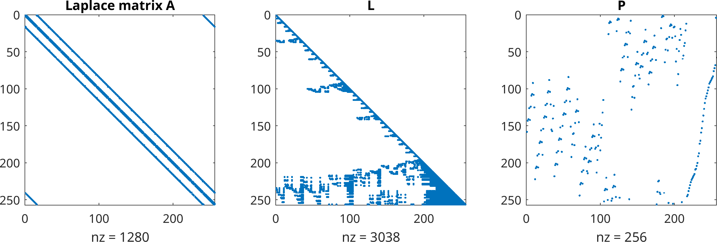
Sparse matrices can also be fully factorized, for example using an LDLt decomposition for the symmetric Laplacian matrix $A=M{\mathrm{\Omega }}^{-1}D$ (used to compute the pressure), or for the diffusion matrix $D$ (useful for implicit time-stepping methods required for larger viscosities). In the case of iterative solvers, obtaining good preconditioners is also easier with matrices, since diagonals can be extracted and partial LU decompositions can be computed.

Sparsity pattern of the Laplace matrix on a 16x16 grid with a periodic domain. The LDLt decomposition (with permutation) is given as PAP' = LDL'. The matrix L is lower diagonal, and the permutation P is optimized for sparsity of L.

Additionally, using sparse matrices made it trivial to extend the Julia implementation with two features: differentiability and running on GPUs. Chain rules are already provided for common matrix operations in Julia. As a result, the matrix implementation could be made reverse-mode differentiable with minimal effort (making sure not to modify arrays anywhere in the computational chain). I use this to optimize closure model coefficients while embedded in the solver. CUDA.jl has all the tools for porting the code to Nvidia GPUs. The code for the matrix assembly was not easy to port, so I ended up doing the assembly on the CPU and transferring the sparse matrices onto the GPU after assembly. The actual solver code was agnostic to the array types used, so no modification was needed there. Solving implicit problems however was a bit more tricky, as I couldn't immediately find good sparse matrix factorization capabilities for the GPU. Initially while porting I did the factorization on the CPU (for solving the pressure Poisson equation), making the actual speed-up much smaller. I also tried iterative solvers, but they were not as fast as using precomputed factorizations. They also require good preconditioners, of which partial LU factorizations are good candidates (but I couldn't find this for CUDA.jl). For fully periodic cases however, the solution to the pressure Poisson equation can be explicitly written down using discrete Fourier transforms, which CUDA.jl supports out of the box. It was very pleasant to see the speed-up. Later I also found CUDSS.jl, which is not included in CUDA.jl. This provides efficient sparse factorizations.

However, I ran into problems when solving for larger 3D problems. Turbulent flows require very fine grids, but GPUs have limited memory. While the sparse matrices contain a lot of redundant information (finite difference stencils), they still require storing all the non-zero coefficients. Since the equations are solved in 2D or 3D, the finite-difference like matrices do not have an obvious multi-diagonal structure, and the only reasonable matrix type are raw sparse matrices. This led me to look into matrix-free methods.

Writing matrix-free operators as kernels

Adding adjoint kernels for differentiability

Next steps

---

1. F. H. Harlow and J. E. Welch. Numerical Calculation of Time‐Dependent Viscous Incompressible Flow of Fluid with Free Surface. The Physics of Fluids 8, 2182–2189 (1965), link. ↩︎