Equivariance

Introduction to GSpaces and FiberFields using the SteerableConvolutions.jl package.

using SteerableConvolutions
using CairoMakie

GSpaces

Create 2-dimensional GSpace with cyclic group of order 4.

G = CyclicGroup(4)
gspace = GSpace(G, 2)

GSpace{CyclicGroup}(CyclicGroup(4), 2)

Fiber fields

We first create a representation.

ρ = Irrep(G, 0) ⊕ Irrep(G, 1)

Representation{Vector{Int64}, Matrix{Float64}}([0, 1], [1.0 0.0 0.0; 0.0 1.0 -0.0; 0.0 0.0 1.0])

Since our fieldtype contains one scalar field (from Irrep(G, 0)) and one 2D-vector field (from Irrep(G, 1)), we need to create a feature field with three channels. We wrap it in a FiberField from a field type and data.

n = 50
grid = LinRange(0, 1, n + 1)
mask = @. (1 - grid^2) * (1 - (grid')^2)
x = zeros(n + 1, n + 1, 3)
@. x[:, :, 1] = sinpi(10 * grid) * mask
@. x[:, :, 2] = sinpi(2 * grid) * cospi(3 * grid') * mask
@. x[:, :, 3] = -cospi(2 * grid) * sinpi(3 * grid') * mask
field = FiberField(gspace, ρ, x)

FiberField{GSpace{CyclicGroup}, Representation{Vector{Int64}, Matrix{Float64}}, Array{Float64, 3}}(GSpace{CyclicGroup}(CyclicGroup(4), 2), Representation{Vector{Int64}, Matrix{Float64}}([0, 1], [1.0 0.0 0.0; 0.0 1.0 -0.0; 0.0 0.0 1.0]), [0.0 0.0 … 0.0 0.0; 0.5875501381915562 0.5873151181362796 … 0.023266985472385673 0.0; … ; -0.023276295990781914 -0.023266985472385603 … -0.0009217413212349656 -0.0; 0.0 0.0 … 0.0 0.0;;; 0.0 0.0 … -0.0 -0.0; 0.12528310027087855 0.1230147665309968 … -0.004873334088262788 -0.0; … ; -0.004963196049146463 -0.004873334088262792 … 0.00019306125439696572 0.0; 0.0 0.0 … -0.0 -0.0;;; -0.0 -0.18730636205989035 … -0.007420300057594717 -0.0; -0.0 -0.18575506369116984 … -0.007358844059794265 -0.0; … ; -0.0 -0.007358844059794257 … -0.0002915268355020542 -0.0; -0.0 -0.0 … -0.0 -0.0])

We now apply a group transform (rotation by 90 degrees):

g = G(1)
newfield = g * field

FiberField{GSpace{CyclicGroup}, Representation{Vector{Int64}, Matrix{Float64}}, Array{Float64, 3}}(GSpace{CyclicGroup}(CyclicGroup(4), 2), Representation{Vector{Int64}, Matrix{Float64}}([0, 1], [1.0 0.0 0.0; 0.0 1.0 -0.0; 0.0 0.0 1.0]), [0.0 0.0 … 0.0 0.0; 0.0 0.023266985472385673 … -0.0009217413212349656 0.0; … ; 0.0 0.5873151181362796 … -0.023266985472385603 0.0; 0.0 0.5875501381915562 … -0.023276295990781914 0.0;;; 0.0 0.0 … 0.0 0.0; 0.007420300057594717 0.007358844059794265 … 0.0002915268355020542 0.0; … ; 0.18730636205989035 0.18575506369116984 … 0.007358844059794257 0.0; 0.0 7.671377386699417e-18 … -3.039081077564003e-19 0.0;;; 0.0 0.0 … 0.0 0.0; -4.543623357123145e-19 -0.004873334088262789 … 0.0001930612543969657 0.0; … ; -1.1469206837828998e-17 0.12301476653099679 … -0.004873334088262793 0.0; 0.0 0.12528310027087855 … -0.004963196049146463 0.0])

Plot the all fields

function plot(field)
    (; x) = field
    s = @. sqrt(field.x[:, :, 2]^2 + field.x[:, :, 3]^2)
    color = s[:] ./ maximum(s)
    limits = (0, 1, 0, 1)
    fig = Figure(; size = (800, 400))
    heatmap(fig[1, 1], grid, grid, x[:, :, 1]; axis = (; limits, title = "Scalar field"))
    arrows(
        fig[1, 2],
        grid,
        grid,
        x[:, :, 2],
        x[:, :, 3];
        lengthscale = 0.1,
        color,
        axis = (; limits, title = "Vector field"),
    )
    fig
end

plot (generic function with 1 method)

Here are the original fields:

plot(field)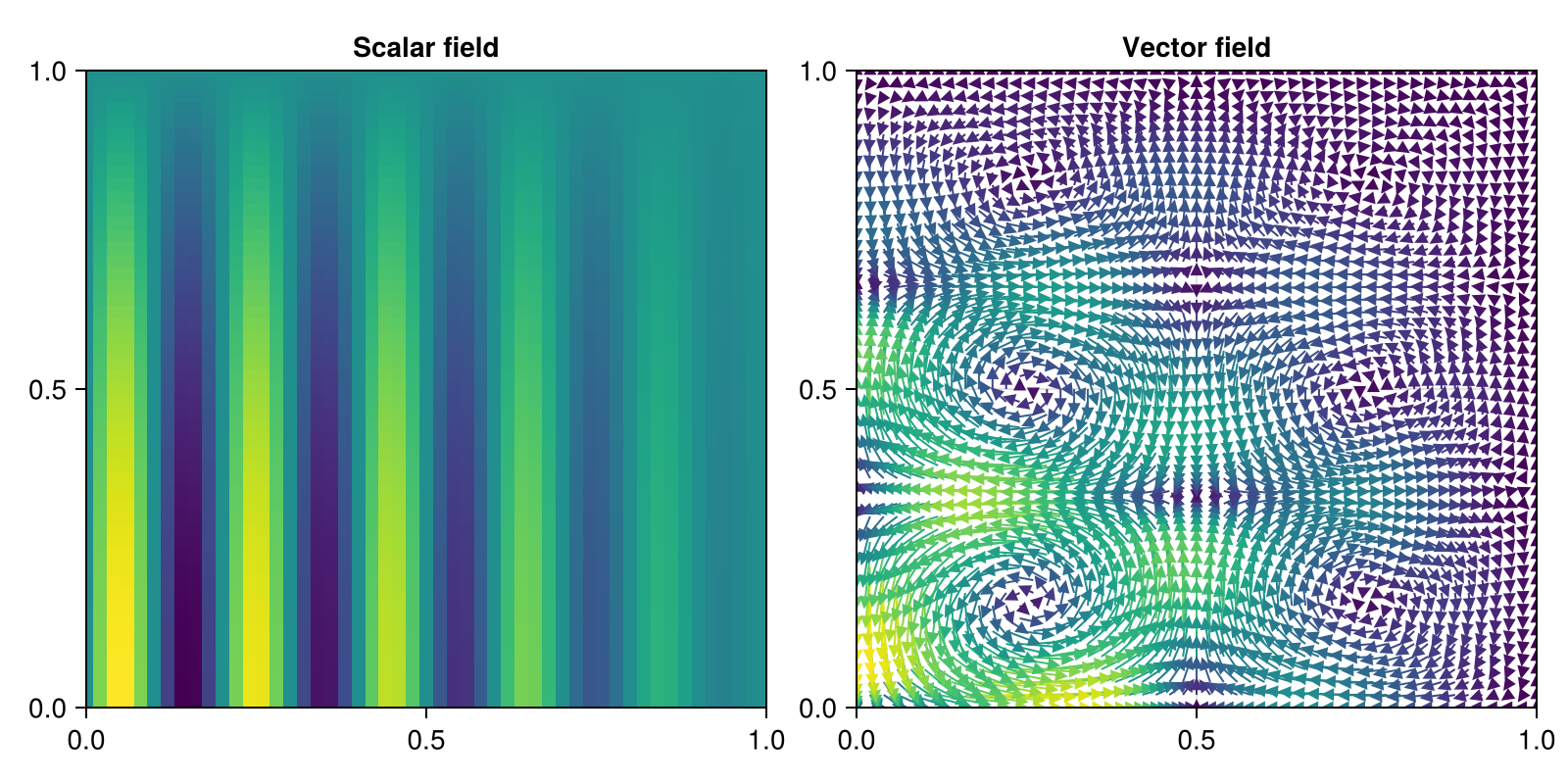

Here are the rotated fields. For the vector field, note also how both the domain and the arrows have been rotated.

plot(newfield)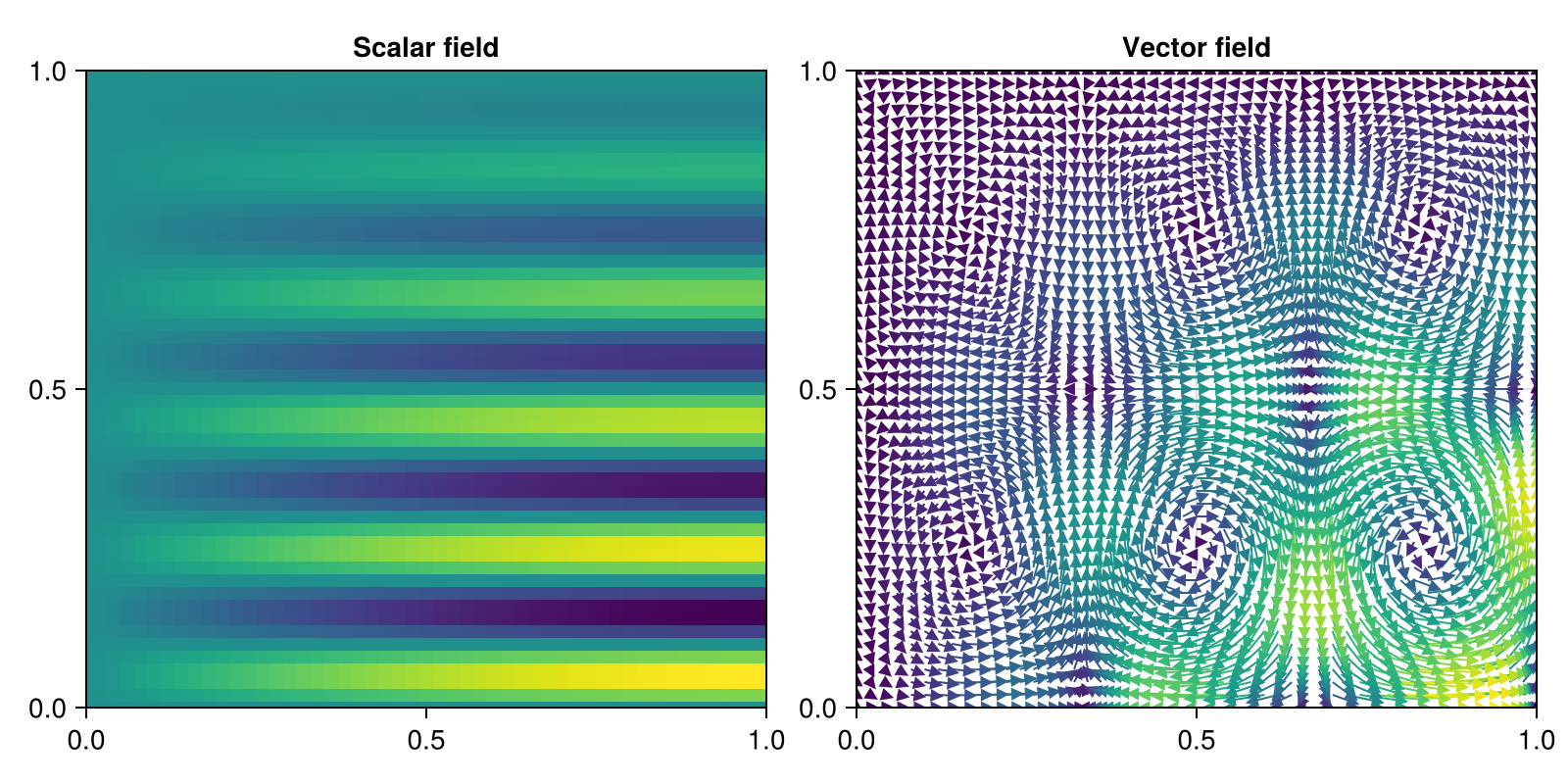

Equivariance

A function $f$ mapping one fiber field $u$ with representation ${\rho }_{\text{in}}$ to another fiber field of representation ${\rho }_{\text{out}}$ is said to be $G$-equivariant if

$$f({\rho }_{\text{in}}(g)u)={\rho }_{\text{out}}(g)f(u)$$

for all $g\in G$.

For example, consider ${\rho }_{\text{in}}$ to be the representation from above, and ${\rho }_{\text{out}}$ to be the trivial representation:

ρ_out = Irrep(gspace.group, 0)

Irrep{CyclicGroup, Int64}(CyclicGroup(4), 0)

The following function is not equivariant:

function notequivariant(u)
    (; x) = u
    y = x[:, :, 2:2] + x[:, :, 3:3]
    FiberField(gspace, ρ_out, y)
end

notequivariant (generic function with 1 method)

since

a = g * notequivariant(field)
b = notequivariant(g * field)
a.x ≈ b.x

false

is false. The following function is equivariant:

function norm2(u)
    (; x) = u
    y = @. x[:, :, 2:2]^2 + x[:, :, 3:3]^2
    FiberField(gspace, ρ_out, y)
end

norm2 (generic function with 1 method)

since

a = g * norm2(field)
b = norm2(g * field)
a.x ≈ b.x

true

---

This page was generated using Literate.jl.