Preserving structure in neural network models

Neural networks are powerful function approximators. Any function $f : \mathbb{R}^n \to \mathbb{R}^m$ can supposedly be approximated to arbitrary accuracy using neural networks. However, approximating $f$ alone is often not sufficient if we want to preserve the properties of $f$. How can those properties be enforced?

Consider the simple case of a linear function

with $A \in \mathbb{R}^{n \times n}$. A three-layer "vanilla" neural network model (multi-layer perceptron with rectified linear units) would look something like

where $\sigma(x) = \max(0, x)$ and $\theta = (B_1, B_2, B_3, b_1, b_2, b_3)$ with $B_1, B_2, B_3 \in \mathbb{R}^{n \times n}$ and $b_1, b_2, b_3 \in \mathbb{R}^{n}$.

Let's define a random reference model and a neural network.

using Random

Random.seed!(0)

n = 5
A = randn(n, n)
f(x) = A * x

σ(x) = max(0, x)
NN(x, (; B₁, B₂, B₃, b₁, b₂, b₃)) = B₃ * σ.(B₂ * σ.(B₁ * x .+ b₁) .+ b₂) .+ b₃

NN (generic function with 1 method)

We will start off with some random parameters. ComponentArrays makes $\theta$ behave both like a very long vector and a named tuple.

using ComponentArrays
θ₀ = ComponentArray(;
    B₁ = randn(n, n),
    B₂ = randn(n, n),
    B₃ = randn(n, n),
    b₁ = randn(n),
    b₂ = randn(n),
    b₃ = randn(n),
);

To measure the performance of our model, we define a "naive" a-priori error measure

and its relative error counterpart

for some random input $x$.

using LinearAlgebra

L(x, θ) = sum(abs2, NN(x, θ) - f(x))
L(θ) = L(randn(n), θ)

xvalid = randn(n)
apriori_error(θ) = norm(NN(xvalid, θ) - f(xvalid)) / norm(f(xvalid))
apriori_error(θ₀)

2.9151871029849366

The initial model is clearly not doing too well. To improve our model, we will perform some iterations of stochastic gradient descent. Luckily, we got Zygote to help us out with the gradients (telling us where to go when we are lost in the dark).

using Zygote

function train(θ; niter = 5_000, η = 0.001, batch_size = 20)
    e = [apriori_error(θ)]
    for i = 1:niter
        g = sum(first(gradient(L, θ)) for _ = 1:batch_size) / batch_size
        θ = θ - η * g
        push!(e, apriori_error(θ))
    end
    θ, e
end

θ, e = train(θ₀);

Let's check how that went.

using Plots
plot(e; label = false, title = "A priori error")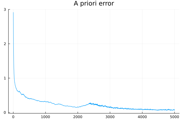

apriori_error(θ)

0.07060941996402383

Not so bad! For the same random input $x$, the models $f$ and $\operatorname{NN}(\cdot, \theta)$ produce almost the same output. But the reference model $f$ is so much more than the mere output it produces, it has structure. In particular, we can always expect $f$ to respect the following properties:

• Additivity:

• Homogeneity:

In other words, $f$ is a linear map. Even though $\operatorname{NN}$ is trained to be really close to $f$, does it have the same linearity properties? Let's check:

x = randn(n)
y = randn(n)
additivity_error = norm(NN(x + y, θ) - NN(x, θ) - NN(y, θ)) / norm(NN(x, θ) + NN(y, θ))

0.029682796633364303

Let's check the scaling properties:

x = randn(n)
homogeneity_error(λ) = norm(NN(λ * x, θ) - λ * NN(x, θ)) / norm(λ * NN(x, θ))
plot(
    LinRange(-10, 10, 100),
    homogeneity_error;
    xlabel = "λ",
    title = "Relative homogeneity error",
    label = false,
)

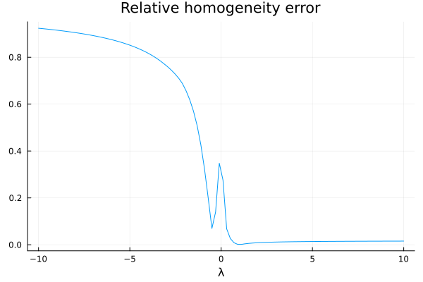
Ouch. We are not doing so well, it seems.

What can we do about this? I can only think of two options:

1. Choosing the parameters $\theta$ more judiciously. In particular, we could change the loss function to penalize deviations from the desired structure in addition to producing correct outputs. We could for example minimize

in the hope of passive-agressively bullying our model towards homogeneity. This idea has popularized the use of things like physics informed neural networks (PINNs), where physical structure (the respect of partial differential equations and their prescribed boundary conditions) are encouraged in the loss function.

2. Choosing the model architecture $\operatorname{NN}$ more judiciously, such that structure is enforced, even before training has occured. In our simple case, where the desired structure is linearity, this would correspond to choosing the alternative model

with $\theta = B_1 \in \mathbb{R}^{n \times n}$. Yes, you read that right. After all, the best possible approximation for a linear model is... a linear model. In particular, we know there exists a very nice parameter set $B_1 = A$, for which our error measures should give some very pleasing values. With a nice training algorithm, dataset, and loss function, we might even be lucky enough to find it.

Conclusion

With large datasets available one might be tempted to learn entire input-output mappings directly, using purely data-driven loss functions. This can be achieved to high accuracy. But enforcing physical structure can be achieved with more careful choices of the model and its parameters. An otherwise unexplainable neural network model that is shown to respect conservation of mass, momentum, and energy is much easier to sell to concerned physicists.